Pome

21.13.1 Toric setupE05D6993D0C8

Let $T$ be a complex torus of dimension $n$ with character lattice $M$ and cocharacter lattice $N$. Some basic terminology is recalled in subsection 21.12.1. Recall that $T_ c$ is the compact torus contained in $T(\mathbb {C})$.

Consider a rational polyhedral fan $\Sigma $ in $N_{\mathbb {R}}$ corresponding to an $n$-dimensional smooth projective toric variety $X$.

Let

\[ D=\sum _{\rho \in \Sigma (1)} a_{\rho }D_{\rho } \]

be a $T$-invariant integral big divisor on $X$. Let $P_ D\subseteq M_{\mathbb {R}}$ be the following polytope1

2A3462C0F498 21.13.2
\begin{equation} P_ D=\left\{ m\in M_{\mathbb {R}}: \langle m,u_{\rho }\rangle \geq -a_{\rho }\quad \forall \rho \in \Sigma (1)\right\} . \end{equation}

Since we have assumed that $D$ is big, $P_ D$ is $n$-dimensional.

Let $L=\mathcal{O}_ X(D)$. Note that replacing $D$ by a linearly equivalent divisor amounts to replacing $P_ D$ by an integral translation.

Recall that for each $\rho \in \Sigma (1)$, $u_{\rho }$ denotes the ray generator of $\rho $. Let $\{ m_{\sigma }\} _{\sigma \in \Sigma }$ denote the Cartier data associated with $D$. In other words, for each $\sigma \in \Sigma $, $m_{\sigma }\in M$ satisfies that

\[ \langle m_{\sigma },u_{\rho } \rangle =-a_{\rho },\quad \forall \rho \in \sigma (1). \]

The element $m_{\sigma }\in M$ is well-defined modulo

077C9BE27980 21.13.3
\begin{equation} M(\sigma )\coloneqq \sigma ^{\perp }\cap M, \end{equation}

where

\[ \sigma ^{\perp }\coloneqq \left\{ m\in M_{\mathbb {R}} : \langle m,u\rangle =0 \quad \forall u\in \sigma \right\} . \]

Moreover, if $\tau $ is a face of $\sigma $, then

88DD52C918D3 21.13.4
\begin{equation} m_{\sigma }\equiv m_{\tau } \mod M(\tau ). \end{equation}

See [Theorem 4.2.8, CLS11]. In particular, for an $n$-dimensional $\sigma \in \Sigma $, the element $m_{\sigma }$ is uniquely determined. In general, for $\sigma \in \Sigma (n)$, one need not have $m_{\sigma }\in P_ D$. In fact, $m_{\sigma }\in P_ D$ for all $\sigma \in \Sigma (n)$ if and only if $D$ is base-point free. See [Theorem 6.1.7, CLS11].

Note that for any $n$-dimensional cone $\sigma $ in $\Sigma $ and any $\rho \in \sigma (1)$, we have

18C40EE2BAB3 21.13.5
\begin{equation} \langle m-m_{\sigma },u_{\rho } \rangle \geq 0,\quad \forall m\in P_ D, \end{equation}

as a consequence of (21.13.2) and the choice of $m_\sigma $.

Recall that

0CCBC0846420 21.13.6
\begin{equation} D|_{U_{\sigma }}=\operatorname{div}(\chi ^{-m_{\sigma }})|_{U_{\sigma }} \end{equation}

for all $\sigma \in \Sigma $, where $U_{\sigma }$ is the affine subvariety of $X$ corresponding to $\sigma $. See [Proposition 4.1.2, CLS11].

Next consider a $T$-invariant irreducible subvariety $Y\subseteq X$. Since $X$ is smooth, so is $Y$. Let $\sigma $ be the cone in $\Sigma $ corresponding to $Y$. We observe that $\sigma $ corresponds to a (possibly empty) face $Q_{\sigma }$ of $P_ D$:

498E343E626C 21.13.7
\begin{equation} Q_{\sigma }=\left\{ m\in P_ D: \langle m,u_{\rho }\rangle =-a_{\rho }\quad \forall \rho \in \sigma (1) \right\} . \end{equation}

The dimension of $\sigma $ is not necessarily equal to the codimension of $Q$ as we will see in example 21.13.15.

We have the following characterization of the base locus of $D$. We are not aware of a direct reference; the result is likely folklore.

Proposition 21.13.8.111BC1BBBDE6 The base locus $\operatorname{Bs}(D)$ (with the reduced complex structure) of $D$ is a toric-invariant (possibly reducible) subvariety given by the union of $V(\tau )$, where $\tau $ runs over elements in $\Sigma $ satisfying the following condition:

0AA0B0B933FC 21.13.9
\begin{equation} a_{\rho }+\langle m, u_{\rho }\rangle >0\quad \textup{for some }\rho \in \tau (1) \end{equation}

for each $m\in M\cap P_ D$.

Here $V(\tau )$ denotes the toric subvariety of $X$ corresponding to $\tau $. In other words,
\[ V(\tau )=\bigcap _{\rho \in \tau (1)} D_{\rho }. \]

Proof. Recall that

\[ \mathrm{H}^0(X,L)\cong \bigoplus _{m\in M\cap P_ D} \mathbb {C}\chi ^ m. \]

See [Proposition 4.3.3, CLS11] for example. So we only need to understand the common zeros of $D+\operatorname{div}\chi ^ m$ for all $m\in M\cap P_ D$. But we know that

\[ D+\operatorname{div}\chi ^ m=\sum _{\rho \in \Sigma (1)} \left( a_{\rho }+\langle m, u_{\rho }\rangle \right) D_{\rho }. \]

Our assertion follows. $\square$

Corollary 21.13.10.0D3DB05576E8 The stable base locus (with the reduced complex structure) of $D$ is a toric-invariant (possibly reducible) subvariety given by the union of the $V(\tau )$'s, where $\tau $ runs over elements in $\Sigma $ satisfying (21.13.9) for each $m\in P_ D$.

Geometrically, the condition means $Q_{\tau }=\varnothing $.

Proof. It follows from proposition 21.13.8 that the stable base locus of $D$ is given by the union of the $V(\tau )$'s, where $\tau $ runs over elements of $\Sigma $ satisfying (21.13.9) for all $m\in M_{\mathbb {Q}}\cap P_ D$. That is,

\[ M_{\mathbb {Q}}\cap \left\{ m\in P_ D : a_{\rho }+\langle m, u_{\rho }\rangle =0\quad \forall \rho \in \tau (1) \right\} =\varnothing . \]

Since the latter part is a rational polytope, this statement is equivalent to

7480F81CDDBD 21.13.11
\begin{equation} \left\{ m\in P_ D : a_{\rho }+\langle m, u_{\rho }\rangle =0\quad \forall \rho \in \tau (1) \right\} =\varnothing . \end{equation}

Our first assertion follows. $\square$

We will keep two examples in mind.

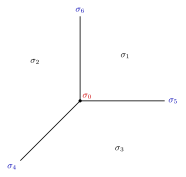
Example 21.13.12.C51FE704A3B3 In this case, $\Sigma $ is the fan in 21.13.13 consisting of three $2$-dimensional cones $\sigma _1$, $\sigma _2$ and $\sigma _3$; three $1$-dimensional cones $\sigma _4$, $\sigma _5$ and $\sigma _6$; one $0$-dimensional cone $\sigma _0$.

Mathematical diagram from the source
85FCE3A7A73121.13.13 The fan $\Sigma $ of $\mathbb {P}^2$. The three rays $\sigma _4,\sigma _5,\sigma _6\in \Sigma (1)$ subdivide $N_{\mathbb {R}}$ into three full-dimensional cones $\sigma _1,\sigma _2,\sigma _3\in \Sigma (2)$; the origin is the unique cone of dimension zero.

The fan $\Sigma $ is just the fan of $X=\mathbb {P}^2$. Under the orbit-cone correspondence, we have

\[ \begin{aligned} D_{\sigma _1}=& \{ [1:0:0]\} ,\quad D_{\sigma _2}=\{ [0:1:0]\} ,\quad D_{\sigma _3}=\{ [0:0:1]\} ,\\ D_{\sigma _4}=& \{ [0:X_1:X_2]:(X_1,X_2)\neq (0,0)\} ,\\ D_{\sigma _5}=& \{ [X_0:0:X_2]:(X_0,X_2)\neq (0,0)\} ,\\ D_{\sigma _6}=& \{ [X_0:X_1:0]:(X_0,X_1)\neq (0,0)\} ,\quad D_{\sigma _0}=\mathbb {P}^2. \end{aligned} \]

In particular, $\Sigma (1)=\{ \sigma _4,\sigma _5,\sigma _6\} $. We shall take

\[ D=D_{\sigma _4}. \]

In other words,

\[ a_{\sigma _5}=a_{\sigma _6}=0,\quad a_{\sigma _4}=1. \]

Note that the ray generators are given by

\[ u_{\sigma _4}=(-1,-1),\quad u_{\sigma _5}=(1,0),\quad u_{\sigma _6}=(0,1). \]

It follows that

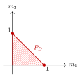
\[ P_ D=\{ m=(m_1,m_2)\in \mathbb {R}^2: m_1+m_2\leq 1, m_1\geq 0, m_2\geq 0\} . \]

Therefore, $P_ D$ is just the polytope in 21.13.14.

Mathematical diagram from the source
16FDB2620E8621.13.14 The polytope $P_ D$.

In this case, the Cartier data for $2$-dimensional cones are given as follows:

\[ m_{\sigma _1}=(0,0),\quad m_{\sigma _2}=(1,0),\quad m_{\sigma _3}=(0,1); \]

while the remaining Cartier data are determined by (21.13.4).

In this case, $L=\mathcal{O}_ X(D)=\mathcal{O}_{\mathbb {P}^2}(1)$. Hence the line bundle $L$ is ample.

We also observe that

\[ \begin{aligned} Q_{\sigma _1}=& \{ (0,0)\} ,\quad Q_{\sigma _2}=\{ (1,0)\} ,\quad Q_{\sigma _3}=\{ (0,1)\} ,\\ Q_{\sigma _4}=& \{ (m_1,m_2):m_1\geq 0,m_2\geq 0,m_1+m_2=1\} ,\\ Q_{\sigma _5}=& \{ 0\} \times [0,1],\quad Q_{\sigma _6}= [0,1]\times \{ 0\} ,\\ Q_{\sigma _0}=& P_ D. \end{aligned} \]
Next we give three non-ample examples.

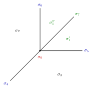
Example 21.13.15.B328D39711DF Let $\Sigma $ be the fan shown in 21.13.16.

Mathematical diagram from the source
C619293CCE8A21.13.16 The fan of $\mathrm{Bl}_0\mathbb {P}^2$. Adding the ray $\sigma _7$ generated by $(1,1)$ subdivides the cone $\sigma _1$ into two full-dimensional cones $\sigma _1',\sigma _1''$.

Comparing with our previous example 21.13.13, we have divided $\sigma _1$ from the middle, giving rise to two additional $2$-dimensional cones $\sigma _1'$ and $\sigma _1''$, and one additional $1$-dimensional cone $\sigma _7$.

The corresponding $X=\mathrm{Bl}_0 \mathbb {P}^2$ is just the blow-up of $\mathbb {P}^2$ at the origin $0=[1:0:0]$ and hence $L=\pi ^*\mathcal{O}_{\mathbb {P}^2}(1)$. Let $\pi \colon X\rightarrow \mathbb {P}^2$ denote the blow-up morphism. Let

\[ D=D_{\sigma _4}. \]

Then $D$ is the pull-back of the divisor $D$ in example 21.13.12. Note that $D$ is not ample, since it has degree $0$ on the exceptional divisor.

In this case, we have

\[ \Sigma (1)=\{ \sigma _4,\sigma _5,\sigma _6,\sigma _7\} , \]

and $D_{\sigma _7}$ is just the exceptional divisor.

The corresponding ray generators are

\[ u_{\sigma _4}=(-1,-1),\quad u_{\sigma _5}=(1,0),\quad u_{\sigma _6}=(0,1),\quad u_{\sigma _7}=(1,1), \]

while

\[ m_{\sigma _1'}=m_{\sigma _1''}=(0,0),\quad m_{\sigma _2}=(1,0),\quad m_{\sigma _3}=(0,1). \]

Therefore, $P_ D$ is the same as in 21.13.14.

We also observe that

\[ \begin{aligned} Q_{\sigma _1'}=& \{ (0,0)\} ,\quad Q_{\sigma _1''}=\{ (0,0)\} ,\quad Q_{\sigma _7}=\{ (0,0)\} ,\\ Q_{\sigma _2}=& \{ (1,0)\} ,\quad Q_{\sigma _3}=\{ (0,1)\} ,\\ Q_{\sigma _4}=& \{ (m_1,m_2):m_1\geq 0,m_2\geq 0,m_1+m_2=1\} ,\\ Q_{\sigma _5}=& \{ 0\} \times [0,1],\quad Q_{\sigma _6}= [0,1]\times \{ 0\} ,\\ Q_{\sigma _0}=& P_ D. \end{aligned} \]

Example 21.13.17.FF229F946E51 We continue with the surface in example 21.13.15 with $X=\mathrm{Bl}_0\mathbb {P}^2$. Let $\pi \colon X\rightarrow \mathbb {P}^2$ be the blow-up morphism, and write

\[ H=D_{\sigma _4},\quad E=D_{\sigma _7}. \]

Consider the toric Cartier divisor

\[ D=2D_{\sigma _4}+D_{\sigma _7}=2H+E. \]

This gives a simple example of a big toric divisor which is not nef.

Indeed, the intersection numbers on $X$ are

\[ H^2=1,\quad H\cdot E=0,\quad E^2=-1. \]

Hence

\[ D\cdot E=(2H+E)\cdot E=-1<0, \]

so $D$ is not nef.

The inequalities defining $P_ D$ are

\[ m_1\geq 0,\quad m_2\geq 0,\quad m_1+m_2\leq 2,\quad m_1+m_2\geq -1. \]

The last inequality, corresponding to the exceptional ray $\sigma _7$, is redundant. This is a typical phenomenon in the non-ample situation. Thus

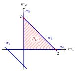
\[ P_ D=\{ m=(m_1,m_2)\in M_{\mathbb {R}}:m_1\geq 0,\ m_2\geq 0,\ m_1+m_2\leq 2\} , \]

as illustrated in 21.13.18.

Mathematical diagram from the source
EFB6C6617A5921.13.18 The polytope $P_ D$ for $D=2D_{\sigma _4}+D_{\sigma _7}$. The blue lines are the four affine hyperplanes $a_{\rho }+\langle m,u_{\rho }\rangle =0$ for $\rho \in \Sigma (1)$.

Example 21.13.19.9A122D0D1FDF We give a surface example in which $P_ D$ is not a lattice polytope. Let $\Sigma $ be the fan in $N_{\mathbb {R}}\simeq \mathbb {R}^2$ whose rays are generated, in cyclic order, by

\[ u_{\rho _1}=(1,0),\quad u_{\rho _2}=(0,1),\quad u_{\rho _3}=(-1,2),\quad u_{\rho _4}=(0,-1). \]

The corresponding smooth projective toric surface is the Hirzebruch surface $\mathbb {F}_2$. Consider the toric Cartier divisor

\[ D=-D_{\rho _3}+2D_{\rho _4}. \]

Thus

\[ a_{\rho _1}=a_{\rho _2}=0,\quad a_{\rho _3}=-1,\quad a_{\rho _4}=2. \]

Hence

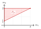
\[ P_ D=\left\{ m=(m_1,m_2)\in M_{\mathbb {R}}: m_1\geq 0,\ \frac{m_1+1}{2}\leq m_2\leq 2 \right\} . \]

See 21.13.20.

Mathematical diagram from the source
BFF7444AF5BE21.13.20 A surface example where $P_ D$ is not a lattice polytope.
Cite this page

Comments

Corrections, questions, and mathematical discussion are welcome. Sign in with GitHub to comment. Comments are public.