Pome

21.12.6 Toric plurisubharmonic functionsE5B138E4CBB0

We continue to use the notations of subsection 21.12.1.

Lemma 21.12.7.1F4ACCC03A78 Let $F\colon N_{\mathbb {R}}\rightarrow [-\infty ,\infty ]$ be a function. Then the following are equivalent:

  1. AB1950E65189

    $F$ is convex and takes values in $\mathbb {R}$, and

  2. AFD8C117A0B0

    $\operatorname{Trop}^*F$ is plurisubharmonic on $T(\mathbb {C})$.

Proof. We may choose an identification $N\cong \mathbb {Z}^ n$ so that we have an identification $T(\mathbb {C})\cong \mathbb {C}^{*n}$. Then $\operatorname{Trop}$ is identified with the map

\[ \operatorname{Trop}\colon \mathbb {C}^{*n}\rightarrow \mathbb {R}^ n,\quad (z_1,\ldots ,z_ n)\mapsto \left(\log |z_1|^2,\ldots ,\log |z_ n|^2\right). \]

1 $\implies $ 2. By the standard convolution regularization of finite convex functions, let $F_ k\in C^{\infty }(\mathbb {R}^ n)\cap \mathrm{Conv}(\mathbb {R}^ n)$ be a decreasing sequence with limit $F$. It follows from a straightforward computation that

836C60871D35 21.12.8
\begin{equation} \begin{split} \mathrm{dd}^{\mathrm{c}}\operatorname{Trop}^*F_ k(z_1,\ldots ,z_ n) =& \frac{\mathrm{i}}{2\pi } \sum _{i,j=1}^ n \partial _{ij}F_ k\left(\log |z_1|^2,\ldots ,\log |z_ n|^2\right)\\ & \times z_ i^{-1}\overline{z_ j}^{-1}\mathrm{d}z_ i\wedge \mathrm{d}\overline{z_ j}. \end{split} \end{equation}

So $\operatorname{Trop}^* F_ k$ is plurisubharmonic. It follows from proposition 5.14.2 that $\operatorname{Trop}^* F$ is plurisubharmonic.

2 $\implies $ 1. It follows from 5.14.14 that $F$ is finite. Moreover, by radial regularization, we may find a decreasing sequence $\varphi _ k$ of $(S^1)^ n$-invariant smooth psh functions on $\mathbb {C}^{*n}$ with limit $\operatorname{Trop}^*F$. Write $\varphi _ k=\operatorname{Trop}^* F_ k$ for some function $F_ k\colon \mathbb {R}^ n\rightarrow \mathbb {R}$; it follows from (21.12.8) that $F_ k$ is convex for all $k$. Therefore, $F$ is convex by 21.11.13. $\square$

Next we define a canonical Kähler form in $c_1(L)$.

Let $G_0\colon M_{\mathbb {R}}\rightarrow (-\infty ,\infty ]$ be defined as

CC04BEE427C7 21.12.9
\begin{equation} G_0(m)\coloneqq \begin{cases} \sum \limits _{\rho \in \Sigma (1)} \left(\langle m, u_{\rho }\rangle +a_{\rho }\right)\log \left(\langle m, u_{\rho }\rangle +a_{\rho }\right){}^{\href{#sgpt-a0000043827}{5}},& \textup{if }m\in P,\\ \infty ,& \textup{otherwise}. \end{cases} \end{equation}

This is a closed proper convex function and $G_0\sim \chi _ P$, where $\sim $ is the relation defined in definition 21.11.19.

Let

AA66EBA79840 21.12.10
\begin{equation} F_0=G_0^* \in \mathcal{E}^{\infty }(N_{\mathbb {R}},P). \end{equation}

Here $G_0^*$ is the Legendre transform of $G_0$, as recalled in definition 21.11.22. The set $\mathcal{E}^{\infty }(N_{\mathbb {R}},P)$ is defined in definition 21.11.41.

By Guillemin's theorem [Gui94, CDG03], $\mathrm{dd}^{\mathrm{c}}\operatorname{Trop}^* F_0$ can be extended to a unique Kähler form $\omega $ in $c_1(L)$. The Kähler form $\omega $ is clearly $T_ c$-invariant.

For each $\rho \in \Sigma (1)$, we write

\[ r_{\rho }(m)=\log \left(\langle m,u_{\rho }\rangle +a_{\rho }\right)+1,\quad m\in P. \]

It follows from (21.12.9) that

C0E06297D5EF 21.12.11
\begin{equation} \nabla G_0(m)=\sum _{\rho \in \Sigma (1)} r_{\rho }(m)u_{\rho },\quad m\in \operatorname{Int}P. \end{equation}

Example 21.12.12.CD7BA5BA48AF Let us move on with our favorite example example 21.12.4. We continue to use the same notations. In this case,

\[ G_0(m)= \begin{cases} m\log m+(1-m)\log (1-m),& \textup{if } m\in [0,1],\\ \infty ,& \textup{otherwise}. \end{cases} \]

The Legendre transform is given by

\[ F_0(n)=\log \left(1+\mathrm{e}^ n\right). \]

Composing with the tropicalization map, we find that

\[ \omega |_{\mathbb {C}^*}(z)=\mathrm{dd}^{\mathrm{c}}\log \left(1+|z|^2\right). \]

This is exactly the Fubini–Study metric as we have seen in example 5.20.6.

We can now explain one subtlety: in our expression (21.12.9), there is no factor $1/2$ before the sum; the absence of the factor $1/2$ matches the choice $\operatorname{Trop}(z)=\log |z|^2$ rather than $\log |z|$ in our tropicalization map (21.12.3).

Let $\mathrm{PSH}_{\mathrm{tor}}(X,\omega )$ denote the set of $T_ c$-invariant $\omega $-psh functions.

Theorem 21.12.13.8B5B73657BF7 There are canonical bijections between the following three sets:

  1. 7680C9B63EAE

    The set of $\varphi \in \mathrm{PSH}_{\mathrm{tor}}(X,\omega )$,

  2. 2C49CA751C18

    the set $\mathcal{P}(N_{\mathbb {R}},P)$ in definition 21.11.41, namely, the set of convex functions $F\colon N_{\mathbb {R}}\rightarrow \mathbb {R}$ satisfying $F\preceq \operatorname{Supp}_ P$, and

  3. B8FE90D4F13F

    the set of closed proper convex functions $G\in \mathrm{Conv}(M_{\mathbb {R}})$ satisfying

    \[ G|_{M_{\mathbb {R}}\setminus P}\equiv \infty . \]
For the notions of closedness and properness, we refer to definition 21.11.3 and definition 21.11.15.

Proof. The bijection between 2 and 3 is the classical Legendre duality. Given $F$ as in 2, we construct $G=F^*$ and vice versa, see proposition 21.11.38.

The map from 1 to 2 is given as follows: Given $\varphi \in \mathrm{PSH}_{\mathrm{tor}}(X,\omega )$, since $\varphi $ is $T_ c$-invariant, we can find $f\colon N_{\mathbb {R}}\rightarrow [-\infty ,\infty )$ such that

0CA6FBB8B2BF 21.12.14
\begin{equation} \varphi |_{T(\mathbb {C})}=\operatorname{Trop}^*f. \end{equation}

We then define $F=f+F_0$. Then $\operatorname{Trop}^* F\in \mathrm{PSH}(T(\mathbb {C}))$. By 21.12.7, $F(n)$ is finite for any $n\in N_{\mathbb {R}}$ and $F$ is convex. Moreover, $F\preceq \operatorname{Supp}_ P$ since $\varphi $ is bounded from above on the compact space $X$ and $F_0\preceq \operatorname{Supp}_ P$.

Conversely, given a map $F\in \mathcal{P}(N_{\mathbb {R}},P)$, then

\[ \operatorname{Trop}^*(F-F_0)\in \mathrm{PSH}\left(T(\mathbb {C}),\omega |_{T(\mathbb {C})}\right). \]

Since $F\preceq \operatorname{Supp}_ P$ and $F_0\sim \operatorname{Supp}_ P$, the difference $F-F_0$ is bounded from above. Hence the corresponding local psh potentials are locally bounded from above near $X\setminus T(\mathbb {C})$. It follows from theorem 5.14.10 that this function can be extended uniquely to an $\omega $-psh function on $X$. The uniqueness of the extension guarantees its $T_ c$-invariance.

The two maps are inverse to each other by construction. $\square$

Given $\varphi \in \mathrm{PSH}_{\mathrm{tor}}(X,\omega )$, we will write $F_{\varphi }$ and $G_{\varphi }$ for the convex functions given by theorem 21.12.13. From the proof, we have the following relations:

40DB9807D05A 21.12.15
\begin{equation} \varphi |_{T(\mathbb {C})}=\operatorname{Trop}^*\left(F_{\varphi }-F_0\right),\quad G_{\varphi }=F_{\varphi }^*. \end{equation}

In particular, $\varphi |_{T(\mathbb {C})}$ is locally bounded. We will frequently use this result without further explanation.

Example 21.12.16.9BDBC1FA226A Let us take our favorite example example 21.12.12 again. We will continue to use the same notations.

Recall that in example 5.20.12 and example 16.3.22, we constructed two $S^1$-invariant functions in $\mathrm{PSH}(X,\omega )$.

We begin with the function $\varphi $ in example 5.20.12. Recall that

\[ \varphi (z)=\log \frac{|z|^2}{|z|^2+1} \]

for $z\in \mathbb {C}$. The function $f\colon \mathbb {R}\rightarrow \mathbb {R}$ in (21.12.14) is therefore

\[ f(n)=\log \frac{\mathrm{e}^{n}}{1+\mathrm{e}^{n}}. \]

Therefore, $F_{\varphi }\colon \mathbb {R}\rightarrow \mathbb {R}$ is

\[ F_{\varphi }(n)=n. \]

Correspondingly, $G_{\varphi }\colon \mathbb {R}\rightarrow \mathbb {R}$ is

\[ G_{\varphi }(m)= \begin{cases} 0,& \textup{if } m=1;\\ \infty ,& \textup{otherwise}. \end{cases} \]

Similarly, if $\psi $ denotes the function in example 16.3.22, then the function $f$ in (21.12.14) is

\[ f(n)= \begin{cases} -\log \left(\mathrm{e}^ n+1 \right)+(-\log (-n))\lor (n+2),& \textup{if } n<-\log 2;\\ 2+\log \frac{\mathrm{e}^{n}}{1+\mathrm{e}^{n}},& \textup{otherwise}. \end{cases} \]

Therefore,

\[ F_{\psi }(n)= \begin{cases} (-\log (-n))\lor (n+2),& \textup{if } n<-\log 2;\\ 2+n,& \textup{otherwise}. \end{cases} \]

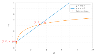
The Legendre transform is tricky to compute. Let $\lambda $ be the large solution of $\log x=x-2$. So $\lambda \approx 3.146$. The smaller solution is around $0.159<\log 2\approx 0.693$. It might be helpful to have a look at the poorly drawn picture 21.12.17.

Mathematical diagram from the source
1AC4B1EDD9A221.12.17 The graphs of $\log x$ and $x-2$.

It is immediate that $G_{\psi }(m)=\infty $ unless $m\in [0,1]$. Let us assume that $m\in [0,1]$. Then

\[ \begin{aligned} G_{\psi }(m)=& \sup _{n\in \mathbb {R}} \left( mn-F_{\psi }(n)\right)\\ =& \sup _{n<-\log 2} \left( mn-(-\log (-n))\lor (n+2)\right) \lor \sup _{n\geq -\log 2} (mn-n-2)\\ =& \sup _{n>\log 2} \left( -mn+(\log n)\land (n-2)\right) \lor \left((1-m)\log 2-2\right). \end{aligned} \]

Let us focus on the first part, which can be decomposed further into

\[ \begin{aligned} & \sup _{n>\log 2} \left( -mn+(\log n)\land (n-2)\right)\\ =& \sup _{n\in \left(\log 2,\lambda \right]} (n-2-mn) \lor \sup _{n>\lambda } (\log n-mn)\\ =& \left( (1-m)\lambda -2 \right) \lor \sup _{n>\lambda } \left(\log n-mn\right). \end{aligned} \]

The latter part can be computed easily:

\[ \sup _{n>\lambda } \left(\log n-mn\right)= \begin{cases} -\log m-1,& \textup{if } m\in \left(0,\lambda ^{-1}\right];\\ \log \lambda -m\lambda ,& \textup{if }m\in \left(\lambda ^{-1},1\right]. \end{cases} \]

Putting everything together, we find

\[ G_{\psi }(m)= \begin{cases} (-\log m-1)\lor \left( (1-m)\lambda -2 \right) ,& \textup{if } m\in \left(0,\lambda ^{-1}\right];\\ (\log \lambda -m\lambda )\lor \left( (1-m)\lambda -2 \right),& \textup{if }m\in \left(\lambda ^{-1},1\right]. \end{cases} \]

This can be further simplified, the final result is

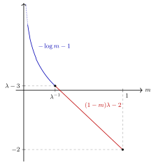
\[ G_{\psi }(m)= \begin{cases} -\log m-1 ,& \textup{if } m\in \left(0,\lambda ^{-1}\right];\\ (1-m)\lambda -2 ,& \textup{if }m\in \left(\lambda ^{-1},1\right];\\ \infty ,& \textup{otherwise}. \end{cases} \]

The graph of $G_{\psi }$ on $(0,1]$ is sketched in 21.12.18.

Mathematical diagram from the source
CC775DD29F7121.12.18 The graph of $G_{\psi }$ on $(0,1]$.
We observe a few elementary facts.

Proposition 21.12.19.EEFA0F6B0CF6 Given $\varphi ,\psi \in \mathrm{PSH}_{\mathrm{tor}}(X,\omega )$. The following are equivalent:

  1. 7C32E25C10B0

    $\varphi \preceq \psi $,

  2. 94A12C520688

    $F_{\varphi }\preceq F_{\psi }$, and

  3. 8A2AEA53E95B

    $G_{\psi }\preceq G_{\varphi }$.

The same holds if we replace all $\preceq $'s by $\leq $.

Proof. The equivalence between 1 and 2 follows from the definition (21.12.15). The equivalence between 2 and 3 follows from the definition of the Legendre transform. $\square$

Similarly, we have

Proposition 21.12.20.D60ADA8CEE9B Given $\varphi \in \mathrm{PSH}_{\mathrm{tor}}(X,\omega )$ and $C\in \mathbb {R}$. We have

\[ F_{\varphi +C}=F_{\varphi }+C,\quad G_{\varphi +C}=G_{\varphi }-C. \]

Proof. The first equality follows from (21.12.15). The second is obtained by taking the Legendre transform. $\square$

Proposition 21.12.21.419A1D9F18A9 Given $\varphi ,\psi \in \mathrm{PSH}_{\mathrm{tor}}(X,\omega )$ with $\varphi \land \psi \not\equiv -\infty $, then $\varphi \land \psi \in \mathrm{PSH}_{\mathrm{tor}}(X,\omega )$ and

\[ F_{\varphi \land \psi }=F_{\varphi }\land F_{\psi },\quad G_{\varphi \land \psi }=G_{\varphi }\lor G_{\psi }. \]
The operators $\land $ and $\lor $ are defined in definition 21.11.10 and definition 21.11.11.

Proof. By proposition 16.3.2, we have $\varphi \land \psi \in \mathrm{PSH}(X,\omega )$. Since $\varphi $ and $\psi $ are $T_ c$-invariant, the set of candidates in the definition of $\varphi \land \psi $ is preserved by the action of $T_ c$. Hence $\varphi \land \psi $ is $T_ c$-invariant as well. So $\varphi \land \psi $ is the biggest element in $\mathrm{PSH}_{\mathrm{tor}}(X,\omega )$ which is dominated by both $\varphi $ and $\psi $. In view of theorem 21.12.13 and proposition 21.12.19, $G_{\varphi \land \psi }$ is the smallest closed proper convex function $G$ on $M_{\mathbb {R}}$ dominating both $G_{\varphi }$ and $G_{\psi }$, which is just $G_{\varphi }\lor G_{\psi }$.

For the statement about $F$, we use proposition 21.11.36:

\[ F_{\varphi \land \psi }=(G_\varphi \lor G_\psi )^*=\operatorname{cl}(F_\varphi \land F_\psi ). \]

Since $\varphi \land \psi \not\equiv -\infty $, $F_{\varphi \land \psi }=(G_\varphi \lor G_\psi )^*$ is finite on all of $N_{\mathbb R}$. It follows that $F_\varphi \land F_\psi >-\infty $, and hence is finite on all of $N_{\mathbb R}$ as well. Being finite and convex on $N_{\mathbb R}$, it is continuous, hence closed. Therefore

\[ F_{\varphi \land \psi }=F_\varphi \land F_\psi . \]
$\square$

Example 21.12.22.2B1E84EAAE13 Now we can give an example of $\varphi ,\psi \in \mathrm{PSH}_{\mathrm{tor}}(X,\omega )$ with $\varphi \land \psi \equiv -\infty $.

We take $P=[0,1]$ so that $X=\mathbb {P}^1$ and $\omega $ is the Fubini–Study metric. Let $\varphi \in \mathrm{PSH}(X,\omega )$ be such that

\[ \varphi (z)=\log \frac{|z|^2}{|z|^2+1} \]

for $z\in \mathbb {C}$. We have computed that $G_{\varphi }$ in example 21.12.16:

\[ G_{\varphi }(m)= \begin{cases} 0,& \textup{if } m=1,\\ \infty ,& \textup{otherwise}. \end{cases} \]

Now we define $\psi \in \mathrm{PSH}_{\mathrm{tor}}(X,\omega )$ as the unique function such that

\[ \psi (z)=\log \frac{1}{|z|^2+1} \]

for $z\in \mathbb {C}$. Then a similar computation shows that

\[ G_{\psi }(m)= \begin{cases} 0,& \textup{if } m=0,\\ \infty ,& \textup{otherwise}. \end{cases} \]

Now we claim that $\varphi \land \psi \equiv -\infty $. Otherwise, we would have

\[ G_{\varphi \land \psi }=G_{\varphi }\lor G_{\psi }\equiv \infty , \]

which is not proper.

Proposition 21.12.23.73034E124A9A Let $\{ \varphi _ i\} _{i\in I}$ be a non-empty family in $\mathrm{PSH}_{\mathrm{tor}}(X,\omega )$ uniformly bounded from above. Then $\operatorname *{sup}_{i\in I}{}\! {}^{*} \varphi _ i\in \mathrm{PSH}_{\mathrm{tor}}(X,\omega )$ and

\[ F_{\operatorname *{sup}_{i\in I}{}\! {}^{*}\varphi _ i}=\bigvee _{i\in I}F_{\varphi _ i},\quad G_{\operatorname *{sup}_{i\in I}{}\! {}^{*}\varphi _ i}=\operatorname{cl}\bigwedge _{i\in I} G_{\varphi _ i}. \]

Moreover, if $I$ is finite, then

\[ G_{\max _{i\in I}\varphi _ i}=\bigwedge _{i\in I} G_{\varphi _ i}. \]

Similarly, if $\{ \varphi _ i\} _{i\in I}$ is a decreasing net in $\mathrm{PSH}_{\mathrm{tor}}(X,\omega )$ such that $\inf _{i\in I}\varphi _ i\not\equiv -\infty $, then $\inf _{i\in I}\varphi _ i\in \mathrm{PSH}_{\mathrm{tor}}(X,\omega )$ and

\[ F_{\inf _{i\in I}\varphi _ i}=\inf _{i\in I}F_{\varphi _ i},\quad G_{\inf _{i\in I}\varphi _ i}=\bigvee _{i\in I}G_{\varphi _ i}. \]
Recall that the closure $\operatorname{cl}$ is defined in definition 21.11.15.

Proof. Thanks to 21.11.13 and proposition 21.11.8, in both cases, the statement for $F$ is clear. The corresponding statement for $G$ is obtained via proposition 21.11.36. When $I$ is finite, the convex function $\bigvee _ i F_{\varphi _ i}$ is finite on all $N_{\mathbb R}$, hence closed. Therefore no additional closure is needed. $\square$

The complex Monge–Ampère operator is closely related to the real one:

Proposition 21.12.24.725063C1ED05 Let $\varphi \in \mathrm{PSH}_{\mathrm{tor}}(X,\omega )$. Then

C2BF3D2E88B4 21.12.25
\begin{equation} \operatorname{Trop}_* \left(\omega |_{T(\mathbb {C})}+\mathrm{dd}^{\mathrm{c}}\varphi |_{T(\mathbb {C})} \right)^ n=\operatorname{MA}_{\mathbb {R}}(F_{\varphi }). \end{equation}

In particular,

\[ \int _ X \omega _{\varphi }^ n =\int _{N_{\mathbb {R}}}\operatorname{MA}_{\mathbb {R}}(F_{\varphi })=n! \operatorname{vol}\overline{\{ G_{\varphi }<\infty \} } \]

and

\[ \int _ X \omega ^ n=n!\operatorname{vol}P. \]
Here the real Monge–Ampère operator is defined in definition 21.11.50. The normalization of the Lebesgue measure $\operatorname{vol}$ on $M_{\mathbb {R}}$ is such that the fundamental lattice cube has measure $1$.6

Proof. We only need to prove (21.12.25). By proposition 21.11.45, we can find a decreasing sequence

\[ F_ j\in \mathcal E^\infty (N_{\mathbb R},P)\cap C^\infty (N_{\mathbb R}) \]

with limit $F_\varphi $. By theorem 21.12.13, each $F_ j$ corresponds to a bounded toric potential $\varphi _ j\in \mathrm{PSH}_{\mathrm{tor}}(X,\omega )$.

By theorem 13.10.4 and theorem 21.11.55, it suffices to establish (21.12.25) for the $\varphi _ j$'s. We may therefore reduce to the case where $F_{\varphi }$ is smooth. We write $F=F_{\varphi }$ to simplify the notations. The notations $a_ i=\log |z_ i|^2$ will be used, where $i=1,\ldots ,n$.

Next we fix an identification $N=\mathbb {Z}^ n$. Fix a test function $f\in C^{0}_ c(N_{\mathbb {R}})$. We need to show that

\[ \int _{\mathbb {C}^{*n}}f(a_1,\ldots ,a_ n) \left(\mathrm{dd}^{\mathrm{c}}\operatorname{Trop}^* F(z_1,\ldots ,z_ n)\right)^ n=\int _{\mathbb {R}^ n} f\, \operatorname{MA}_{\mathbb {R}}(F). \]

Using proposition 21.11.52 and (21.12.8), this reduces to

E34E6BC222DC 21.12.26
\begin{equation} \begin{split} \left( \frac{\mathrm{i}}{2\pi }\right)^ n\int _{\mathbb {C}^{*n}}f(a_1,\ldots ,a_ n) \left(\sum _{i,j=1}^ n \partial _{i,j}F(a_1,\ldots ,a_ n)z_ i^{-1}\overline{z_ j}^{-1}\mathrm{d}z_ i\wedge \mathrm{d}\overline{z_ j}\right)^ n=\\ n!\int _{\mathbb {R}^ n} f \det \nabla ^2 F\, \mathrm{d}\operatorname{vol}. \end{split} \end{equation}

Expanding the bracket, we get

\[ \begin{aligned} \left(\sum _{i,j=1}^ n \partial _{i,j}Fz_ i^{-1}\overline{z_ j}^{-1}\mathrm{d}z_ i\wedge \mathrm{d}\overline{z_ j}\right)^ n =& \sum _{i_1,\ldots ,i_ n=1}^ n \sum _{j_1,\ldots ,j_ n=1}^ n \partial _{i_1j_1}F\cdots \partial _{i_ nj_ n}F\cdot \\ & \mathrm{d}\log z_{i_1}\wedge \mathrm{d}\log \overline{z_{j_1}}\wedge \cdots \wedge \mathrm{d}\log z_{i_ n}\wedge \mathrm{d}\log \overline{z_{j_ n}}, \end{aligned} \]

where $\mathrm{d}\log z_ i=z_ i^{-1}\mathrm{d}z_ i$ and $\mathrm{d}\log \overline{z_ i}=\overline{z_ i}^{-1}\mathrm{d}\overline{z_ i}$ are understood.

Using the apparent symmetry, the expression on the right-hand side becomes

\[ \begin{aligned} & \sum _{\sigma ,\tau \in \mathfrak {S}_ n}\prod _{k=1}^ n \partial _{\sigma (k)\tau (k)}F\, \mathrm{d}\log z_{\sigma (1)}\wedge \mathrm{d}\log \overline{z_{\tau (1)}}\wedge \cdots \wedge \mathrm{d}\log z_{\sigma (n)}\wedge \mathrm{d}\log \overline{z_{\tau (n)}},\\ =& n!\sum _{\tau \in \mathfrak {S}_ n}\prod _{k=1}^ n \partial _{k\tau (k)}F\, \mathrm{d}\log z_{1}\wedge \mathrm{d}\log \overline{z_{\tau (1)}}\wedge \cdots \wedge \mathrm{d}\log z_{n}\wedge \mathrm{d}\log \overline{z_{\tau (n)}}\\ =& n!\sum _{\tau \in \mathfrak {S}_ n}\operatorname {sgn}(\tau )\prod _{k=1}^ n \partial _{k\tau (k)}F\, \mathrm{d}\log z_{1}\wedge \mathrm{d}\log \overline{z_1}\wedge \cdots \wedge \mathrm{d}\log z_{n}\wedge \mathrm{d}\log \overline{z_ n}\\ =& n! \det \nabla ^2 F\mathrm{d}\log z_{1}\wedge \mathrm{d}\log \overline{z_1}\wedge \cdots \wedge \mathrm{d}\log z_{n}\wedge \mathrm{d}\log \overline{z_ n}, \end{aligned} \]

where $\mathfrak {S}_ n$ is the permutation group on $\{ 1,\ldots ,n\} $ and $\operatorname {sgn}(\tau )$ is the sign of $\tau $.

Next, switch to polar coordinates for each $z_ i$: Let $z_ i=r_ i\exp (\mathrm{i}\theta _ i)$ and recall that $r_ i=\exp (a_ i/2)$. Then the left-hand side of (21.12.26) becomes

\[ \begin{split} & \frac{n!}{(2\pi )^ n}\int _{\mathbb {R}^ n\times [0,2\pi )^ n} f \det \nabla ^2 F \, \mathrm{d}a_1\wedge \mathrm{d}\theta _1\wedge \cdots \wedge \mathrm{d}a_ n\wedge \mathrm{d}\theta _ n\\ =& n!\int _{\mathbb {R}^ n}f\det \nabla ^2 F \, \mathrm{d}a_1\wedge \cdots \wedge \mathrm{d}a_ n, \end{split} \]

which is exactly what we have expected. $\square$

Next we study the envelope operators developed in section 16.1 in the toric setting.

Definition 21.12.27.CC64AE504A19 Let $\varphi \in \mathrm{PSH}_{\mathrm{tor}}(X,\omega )$. We define its Newton body as

\[ \Delta (\omega ,\varphi )\coloneqq \overline{\{ G_{\varphi }<\infty \} }\subseteq P. \]

Note that $\Delta (\omega ,\varphi )$ is a convex body.

By proposition 21.11.34, we have
\[ \Delta (\omega ,\varphi )=\overline{\nabla F_{\varphi }(N_{\mathbb {R}})}. \]

Example 21.12.28.E6289865C7A4 By (21.12.9), we have

\[ \Delta (\omega ,0)=P. \]

In the case of example 21.12.16, we have

\[ \Delta (\omega ,\varphi )=\{ 1\} ,\quad \Delta (\omega ,\psi )=[0,1]. \]

Observe that in the latter case,

\[ \{ G_{\psi }<\infty \} \subsetneq P. \]

Proposition 21.12.29.11748980D2DF Let $\varphi \in \mathrm{PSH}_{\mathrm{tor}}(X,\omega )$. Then $P_{\omega }[\varphi ]\in \mathrm{PSH}_{\mathrm{tor}}(X,\omega )$ and

F8C4AC16B8F2 21.12.30
\begin{equation} G_{P_{\omega }[\varphi ]}(x)= \begin{cases} G_0(x),& \textup{if } x\in \Delta (\omega ,\varphi );\\ \infty ,& \textup{otherwise}. \end{cases} \end{equation}

Proof. By (16.3.7), we have

\[ P_{\omega }[\varphi ]=\operatorname *{sup}_{C\in \mathbb {R}}{}\! {}^{*}\bigl ((\varphi +C)\land 0\bigr ). \]

It follows from proposition 21.12.20, proposition 21.12.21 and proposition 21.12.23 that $P_{\omega }[\varphi ]\in \mathrm{PSH}_{\mathrm{tor}}(X,\omega )$. Moreover, by the same propositions, we have

\[ G_{P_{\omega }[\varphi ]}=\operatorname{cl}\inf _{C\in \mathbb {R}} \left( G_{0}\lor (G_{\varphi }-C) \right). \]

We spell out the last closure. Set

\[ K=\inf _{C\in \mathbb {R}} \left( G_{0}\lor (G_{\varphi }-C) \right). \]

If $x\in \operatorname{Dom}G_{\varphi }$, then $G_{\varphi }(x)-C\leq G_0(x)$ for $C$ large enough, hence $K(x)=G_0(x)$. If $x\notin \operatorname{Dom}G_{\varphi }$, then $K(x)=\infty $. Since $\Delta (\omega ,\varphi )=\overline{\operatorname{Dom}G_{\varphi }}$ and $G_0$ is continuous on $P$, the lower semicontinuous regularization $\operatorname{cl}K$ is equal to $G_0$ on $\Delta (\omega ,\varphi )$ and equal to $\infty $ outside $\Delta (\omega ,\varphi )$. This is exactly (21.12.30). $\square$

Recall that $\mathrm{H}^0(X,L)$ can be identified with the vector space generated by $\chi ^ m$ for all $m\in P\cap M$, see Theorem 21.9.5. In other words, a character $\chi ^ m$ of $T$ gives a global section of $L$ if and only if $m\in P$. This gives a beautiful characterization of the lattice points in $P$. The following theorem of Yi Yao gives an analogous characterization of the lattice points in the Newton body.

Theorem 21.12.31 (Yao).E109952155FB Let $\varphi \in \mathrm{PSH}_{\mathrm{tor}}(X,\omega )$. Let $m\in M$.

  1. DB04A0B2F10F

    Suppose that $m\in \Delta (\omega ,\varphi )$. Then $\chi ^ m\in \mathrm{H}^0(X,L\otimes \mathcal{I}(\varphi ))$.

  2. CD5C29228E06

    Let $\sigma \in \Sigma $ be a cone of dimension $p$, with rays $\rho _1,\ldots ,\rho _ p$. Let $c_1,\ldots ,c_ p>0$ satisfy $\sum _{i=1}^ p c_ i=1$, and set $u=\sum _{i=1}^ p c_ i u_{\rho _ i}$. If

    C40469D9226B 21.12.32
    \begin{equation} \langle m,-u\rangle -\operatorname{Supp}_{\Delta (\omega ,\varphi )}(-u)>1, \end{equation}

    then $\chi ^ m\not\in \mathrm{H}^0(X,L\otimes \mathcal{I}(\varphi ))$.

In 2, there are exactly $p$ rays in $\sigma (1)$ since $\sigma $ is smooth.

Proof. Put $\Delta =\Delta (\omega ,\varphi )$. By proposition 16.6.18, proposition 21.12.29, we may replace $\varphi $ by $P_{\omega }[\varphi ]$ without changing its multiplier ideal or Newton body. We may therefore assume that $F_{\varphi }-\operatorname{Supp}_{\Delta }$ is bounded on $N_{\mathbb {R}}$. Set

\[ H(\nu )=\langle m,\nu \rangle -\operatorname{Supp}_{\Delta }(\nu ),\quad \nu \in N_{\mathbb {R}}. \]

Since $\Delta $ is compact, $H$ is Lipschitz and positively homogeneous.

Observe also that $\mathrm{H}^0(X,L\otimes \mathcal{I}(\varphi ))$ is a $T_ c$-invariant subspace of $\mathrm{H}^0(X,L)$. Since the $T_ c$-weight spaces in $\mathrm{H}^0(X,L)$ are the lines $\mathbb {C}\chi ^ m$, it is the direct sum of suitable $\mathbb {C}\chi ^ m$'s.

If $m\notin P$, then $\chi ^ m$ is not a section of $L$. Suppose henceforth that $m\in M\cap P$. Membership in $\mathrm{H}^0(X,L\otimes \mathcal{I}(\varphi ))$ is equivalent to the finiteness of

39F3ED71C89D 21.12.33
\begin{equation} \int _{T(\mathbb {C})}|\chi ^ m|^2\exp (-\operatorname{Trop}^*F_0-\varphi )\, \omega ^ n. \end{equation}

Since $\operatorname{Trop}^*F_0+\varphi =\operatorname{Trop}^*F_{\varphi }$, the boundedness of $F_{\varphi }-\operatorname{Supp}_{\Delta }$ and proposition 21.12.24 show that this is equivalent to the finiteness of

\[ \int _{N_{\mathbb {R}}}\exp (H(\nu ))\, \operatorname{MA}_{\mathbb {R}}(F_0)(\nu ). \]

Changing variables by $\nu =\nabla G_0(m')$, we obtain the equivalent integral

428CD3ABF6EF 21.12.34
\begin{equation} \int _ P\exp \left(\langle m,\nabla G_0(m')\rangle -\operatorname{Supp}_{\Delta }(\nabla G_0(m'))\right)\, \mathrm{d}m'. \end{equation}

If $m\in \Delta $, its integrand is at most $1$, proving 1.

To prove 2, extend $\sigma $ to a maximal cone $\tau \in \Sigma $. Its primitive ray generators $u_1,\ldots ,u_ n$ form a basis of $N$, and we may arrange that $u_ i=u_{\rho _ i}$ for $1\leq i\leq p$. If $e_1,\ldots ,e_ n$ is the dual basis of $M$, then $z_ i=\chi ^{e_ i}$ are coordinates on the affine chart $U_{\tau }\cong \mathbb {C}^ n$.

Let $v\in P\cap M$ be the vertex corresponding to $\tau $. The character $\chi ^ v$ is a local frame of $L$ on $U_{\tau }$. Writing

\[ \nu =\operatorname{Trop}(z)=\sum _{i=1}^ n\log |z_ i|^2\, u_ i, \]

the weight of the singular metric in this frame is $F_{\varphi }(\nu )-\langle v,\nu \rangle $. The local representative of $\chi ^ m$ is $\chi ^{m-v}$, so its squared norm is

\[ \exp \left(\langle m,\nu \rangle -F_{\varphi }(\nu )\right). \]

On the unit polydisc, $\omega ^ n$ is comparable to Euclidean volume. Set $t_ i=-\log |z_ i|^2$. Integrating out the angular variables and using the boundedness of $F_{\varphi }-\operatorname{Supp}_{\Delta }$, the weighted integral over this polydisc is finite if and only if the following integral is finite:

\[ \int _{[0,\infty )^ n}\exp \left(H\left(-\sum _{i=1}^ n t_ i u_ i\right)-\sum _{i=1}^ n t_ i\right)\, \mathrm{d}t. \]

Restrict this integral to the tube parametrized by $s>1$ and $0<y_ i<1$ for $2\leq i\leq n$, with

\[ t_1=c_1s,\qquad t_ i=c_ is+y_ i\quad (2\leq i\leq p),\qquad t_ i=y_ i\quad (p<i\leq n). \]

The Jacobian is $c_1>0$. Since $H$ is Lipschitz and positively homogeneous and $\sum _{i=1}^ p c_ i=1$, the exponent on this tube is

\[ H\left(-\sum _{i=1}^ n t_ i u_ i\right)-\sum _{i=1}^ n t_ i =s\bigl (H(-u)-1\bigr )+\mathcal{O}(1), \]

with a bounded error uniform in $s$ and the $y_ i$'s. The local integral is therefore bounded from below by a positive multiple of

\[ \int _1^{\infty }\exp \left(s\bigl (H(-u)-1\bigr )\right)\, \mathrm{d}s, \]

which diverges under (21.12.32). This proves 2. $\square$

Corollary 21.12.35.05A4124B7E31 Let $\varphi \in \mathrm{PSH}_{\mathrm{tor}}(X,\omega )$. Then

\[ \lim _{k\to \infty }\frac{n!}{k^ n}h^0\left(X,L^ k\otimes \mathcal{I}(k\varphi )\right)= n!\operatorname{vol}\Delta (\omega ,\varphi ). \]

Proof. Take $k>0$. Let $F_{0,k}$ denote the Guillemin potential associated with the polytope $kP$. On $T(\mathbb C)$, set

\[ \widetilde\varphi _ k=\operatorname{Trop}^*(kF_\varphi -F_{0,k}). \]

Then $\widetilde\varphi _ k$ is the toric potential, with respect to the reference metric associated with $kP$, corresponding to the singular metric $h^ k\exp (-k\varphi )$ on $L^ k$. It differs from $k\varphi $ by the smooth toric function $\operatorname{Trop}^*(kF_0-F_{0,k})$. Hence

\[ \mathcal I(\widetilde\varphi _ k)=\mathcal I(k\varphi ). \]

Moreover, the convex function associated with $\widetilde\varphi _ k$ is $kF_\varphi $, so its Legendre transform is

\[ (kF_\varphi )^*(m)=kG_\varphi (m/k). \]

Thus the Newton body of $\widetilde\varphi _ k$ is $k\Delta (\omega ,\varphi )$.

Applying theorem 21.12.31 1 to the line bundle $L^ k$ and the potential $k\varphi $, whose Newton body is $k\Delta (\omega ,\varphi )$, we have

\[ \# \left( k\Delta (\omega ,\varphi )\cap M\right)\leq h^0\left(X,L^ k\otimes \mathcal{I}(k\varphi )\right). \]

Here $\# $ denotes the number of elements. Therefore,

\[ \lim _{k\to \infty }k^{-n}\# \left( k\Delta (\omega ,\varphi )\cap M\right)\leq \varliminf _{k\to \infty } k^{-n} h^0\left(X,L^ k\otimes \mathcal{I}(k\varphi )\right). \]

The left-hand side is just $\operatorname{vol}\Delta (\omega ,\varphi )$, as follows from theorem 19.7.20. So we conclude that

\[ \varliminf _{k\to \infty }\frac{n!}{k^ n}h^0\left(X,L^ k\otimes \mathcal{I}(k\varphi )\right)\geq n!\operatorname{vol}\Delta (\omega ,\varphi ). \]

It remains to prove the reverse inequality.

We choose an identification $M\cong \mathbb {Z}^ n$. In particular, there is a natural distance $\mathrm{d}$ on $M_{\mathbb {R}}\cong \mathbb {R}^ n$. Given a convex body $K$ and $\epsilon >0$, we let

\[ K^{\epsilon }\coloneqq \left\{ x\in \mathbb {R}^ n: \mathrm{d}(x,K)\leq \epsilon \right\} . \]

This is again a convex body, since it can be realized as the Minkowski sum of $K$ with a closed ball of radius $\epsilon $.

Applying theorem 21.12.31 2 to the polytope $kP$ and the potential $\widetilde\varphi _ k$, we can find $C>0$ uniform in $k$ such that for each $k\in \mathbb {Z}_{>0}$,

\[ \bigl \{ m\in M:\chi ^ m\in \mathrm{H}^0(X,L^ k\otimes \mathcal{I}(k\varphi ))\bigr \} \subseteq \left(k\Delta (\omega ,\varphi )\right)^ C. \]

Indeed, if a point $m\in kP\cap M$ is at distance at least $C$ from $k\Delta (\omega ,\varphi )$, the separating hyperplane theorem gives a unit vector $v\in N_{\mathbb R}$ such that

\[ \langle m,v\rangle -\operatorname{Supp}_{k\Delta (\omega ,\varphi )}(v)\geq C. \]

Since the fan $\Sigma $ is finite and covers $N_{\mathbb R}$, there is a constant $\Lambda >0$ with the following property: every unit vector $v\in N_{\mathbb R}$ can be written in the form

\[ v=-\lambda \sum _ i c_ i u_{\rho _ i},\quad 0<\lambda \leq \Lambda ,\quad c_ i>0,\quad \sum _ i c_ i=1, \]

where the rays $\rho _ i$ are contained in a single cone of $\Sigma $. Put

\[ u\coloneqq \sum _ i c_ i u_{\rho _ i}. \]

Since the support function is positively homogeneous, we have

\[ \begin{aligned} \langle m,-u\rangle -\operatorname{Supp}_{k\Delta (\omega ,\varphi )}(-u)& =\lambda ^{-1}\left(\langle m,v\rangle -\operatorname{Supp}_{k\Delta (\omega ,\varphi )}(v)\right)\\ & \geq C/\Lambda . \end{aligned} \]

Choosing $C>\Lambda $ makes (21.12.32) applicable, uniformly in $k$.

Fix $\epsilon >0$. Then for large enough $k$, we have

\[ \left(k\Delta (\omega ,\varphi )\right)^{C}\subseteq k\left(\Delta (\omega ,\varphi )^{\epsilon }\right). \]

It follows that

\[ h^0\left(X,L^ k\otimes \mathcal{I}(k\varphi )\right)\leq \# \left( k\left(\Delta (\omega ,\varphi )^{\epsilon }\right) \cap M\right). \]

Applying theorem 19.7.20 again, we conclude that

\[ \varlimsup _{k\to \infty } \frac{n!}{k^ n} h^0\left(X,L^ k\otimes \mathcal{I}(k\varphi )\right)\leq n! \operatorname{vol}\left(\Delta (\omega ,\varphi )^{\epsilon }\right). \]

Letting $\epsilon \to 0+$ and applying theorem 19.7.5, we find

\[ \varlimsup _{k\to \infty } \frac{n!}{k^ n} h^0\left(X,L^ k\otimes \mathcal{I}(k\varphi )\right)\leq n! \operatorname{vol}\Delta (\omega ,\varphi ). \]

Our assertion follows. $\square$

Example 21.12.36.37CEF2EAED80 In general, in the setup of theorem 21.12.31, there exists $m\in M\cap (P\setminus \Delta (\omega ,\varphi ))$ such that $\chi ^ m\in \mathrm{H}^0(X,L\otimes \mathcal{I}(\varphi ))$.

As a concrete example, let us take $P=[0,1]$. Take $\varphi $ so that $\Delta (\omega ,\varphi )=[0,1/2]$. We claim that $\chi ^1$ is $L^2$-integrable.

It suffices to verify the convergence of (21.12.34). Recall that

\[ \nabla G_0(m')=\log \frac{m'}{1-m'},\quad m'\in [0,1], \]

while

\[ \operatorname{Supp}_{[0,1/2]}(a)= \begin{cases} a/2,& \textup{if }a>0;\\ 0,& \textup{otherwise}. \end{cases} \]

Therefore, (21.12.34) becomes

\[ \int _0^{1/2} \frac{m'}{1-m'}\, \mathrm{d}m'+\int _{1/2}^1 \left(\frac{m'}{1-m'}\right)^{1/2}\, \mathrm{d}m'<\infty . \]
We interpret various classes of potentials studied in 16.5 in the toric setting.

Proposition 21.12.37.852502204924 Let $\varphi \in \mathrm{PSH}_{\mathrm{tor}}(X,\omega )$. Then the following are equivalent:

  1. 9E56D59BF68F

    $\varphi \in \mathcal{E}^{\infty }(X,\omega )$;

  2. E9419C789E2A

    $F_{\varphi }\in \mathcal{E}^{\infty }(N_{\mathbb {R}},P)$;

  3. DC7FED6558A9

    $G_{\varphi }\sim G_0$.

The notation $\mathcal{E}^{\infty }(N_{\mathbb {R}},P)$ is defined in definition 21.11.41.

Proof. This follows immediately from proposition 21.12.19. $\square$

Proposition 21.12.38.55BFC442EA72 Let $\varphi \in \mathrm{PSH}_{\mathrm{tor}}(X,\omega )$. Then the following are equivalent:

  1. 323127E50410

    $\varphi \in \mathcal{E}(X,\omega )$;

  2. BCA447CA7659

    $F_{\varphi }\in \mathcal{E}(N_{\mathbb {R}},P)$;

  3. E488FC604B8A

    $\overline{\operatorname{Dom}G_{\varphi }}=P$.

The notation $\mathcal{E}(N_{\mathbb {R}},P)$ is defined in definition 21.11.41.

Proof. 1 $\iff $ 3. By proposition 21.12.24,

\[ \int _ X \omega _{\varphi }^ n=\int _{T(\mathbb {C})} \left(\omega |_{T(\mathbb {C})}+\mathrm{dd}^{\mathrm{c}}\varphi |_{T(\mathbb {C})} \right)^ n= n! \operatorname{vol}\overline{\operatorname{Dom}G_{\varphi }},\quad \int _ X \omega ^ n=n!\operatorname{vol}P, \]

where in the first equality, we use the fact that $\omega _{\varphi }^ n$ does not charge pluripolar sets proposition 13.11.4 4.

Therefore, 1 and 3 are equivalent.

2 $\iff $ 3. This follows from proposition 21.11.34. $\square$

Proposition 21.12.39.75730375E037 Let $\varphi \in \mathrm{PSH}_{\mathrm{tor}}(X,\omega )$. Then

F02AE1451B98 21.12.40
\begin{equation} E_{\omega }(\varphi )=n!\int _ P \left(G_{0}-G_{\varphi }\right)\, \mathrm{d}\operatorname{vol}. \end{equation}

Proof. For $\psi \in \mathrm{PSH}_{\mathrm{tor}}(X,\omega )$, write

\[ \mathcal C(\psi )\coloneqq n!\int _ P\left(G_0-G_\psi \right)\, \mathrm{d}\operatorname{vol}. \]

Step 1. We assume that $\varphi $ is bounded.

Put $h=F_{\varphi }-F_0$, $\varphi _ t=t\varphi $ and

\[ F_ t\coloneqq F_0+th \]

for $t\in [0,1]$. Then $F_ t=F_{\varphi _ t}$ and $G_ t\coloneqq F_ t^*=G_{\varphi _ t}$. Since $\varphi $ is bounded, $h$ is bounded and continuous; in particular, $F_ t\in \mathcal E^\infty (N_{\mathbb R},P)$ for every $t\in [0,1]$.

We claim that

3654D70C9AC4 21.12.41
\begin{equation} \frac{\mathrm d}{\mathrm dt}\mathcal C(\varphi _ t)=\int _{N_{\mathbb R}}h\, \operatorname{MA}_{\mathbb R}(F_ t). \end{equation}

Let $s>0$ and $t,t+s\in [0,1]$. At a point $m\in \operatorname{Int}P$ where both $G_ t$ and $G_{t+s}$ are differentiable, we have

\[ \begin{aligned} G_{t+s}(m)& \geq G_ t(m)-s h\bigl (\nabla G_ t(m)\bigr ),\\ G_ t(m)& \geq G_{t+s}(m)+s h\bigl (\nabla G_{t+s}(m)\bigr ). \end{aligned} \]

Therefore,

\[ h\bigl (\nabla G_{t+s}(m)\bigr )\leq \frac{G_ t(m)-G_{t+s}(m)}{s}\leq h\bigl (\nabla G_ t(m)\bigr ). \]

Integrating the last inequality and using 21.11.57 gives

\[ \int _{N_{\mathbb R}}h\, \operatorname{MA}_{\mathbb R}(F_{t+s})\leq \frac{\mathcal C(\varphi _{t+s})-\mathcal C(\varphi _ t)}{s}\leq \int _{N_{\mathbb R}}h\, \operatorname{MA}_{\mathbb R}(F_ t). \]

Letting $s\to 0+$ and using theorem 21.11.55 for $F_{t+s}\to F_ t$, we obtain the right derivative in (21.12.41). The left derivative follows in the same way. Hence (21.12.41) holds.

By proposition 21.12.24, the right-hand side of (21.12.41) is

\[ \int _ X\varphi \, \omega _{\varphi _ t}^ n. \]

On the other hand, 16.5.57 gives

\[ \frac{\mathrm d}{\mathrm dt}E_{\omega }(\varphi _ t)=\int _ X\varphi \, \omega _{\varphi _ t}^ n. \]

Thus $E_{\omega }(\varphi _ t)-\mathcal C(\varphi _ t)$ is constant in $t$. It vanishes at $t=0$, hence (21.12.40) follows by taking $t=1$.

Step 2. We handle the general case.

Both sides of (21.12.40) change by the same additive constant when we replace $\varphi $ by $\varphi +A$, namely by

\[ A\int _ X\omega ^ n=A\, n!\operatorname{vol}P. \]

We may therefore assume that $\varphi \leq 0$. For $C>0$, put

\[ \varphi _ C\coloneqq \varphi \lor (-C). \]

Then $\varphi _ C\in \mathrm{PSH}_{\mathrm{tor}}(X,\omega )\cap L^{\infty }(X)$ and $\varphi _ C\searrow \varphi $ as $C\to \infty $. By proposition 21.12.23, $G_{\varphi _ C}\nearrow G_{\varphi }$. Applying Step 1 to $\varphi _ C$, we get

\[ E_{\omega }(\varphi _ C)=n!\int _ P \left(G_0-G_{\varphi _ C}\right)\, \mathrm{d}\operatorname{vol}. \]

Letting $C\to \infty $, the left-hand side converges to $E_{\omega }(\varphi )$ by proposition 16.5.20. On the right-hand side, since $\varphi _ C\leq 0$, we have $G_{\varphi _ C}\geq G_0$, and the monotone convergence theorem applied to $G_{\varphi _ C}-G_0\nearrow G_{\varphi }-G_0$ gives (21.12.40). $\square$

Corollary 21.12.42.E80DDB8667C8 Let $\varphi \in \mathrm{PSH}_{\mathrm{tor}}(X,\omega )$. Then the following are equivalent:

  1. 8FB62A15E0CB

    $\varphi \in \mathcal{E}^1(X,\omega )$;

  2. 055DBC443927

    $F_{\varphi }\in \mathcal{E}^1(N_{\mathbb {R}},P)$;

  3. 97AB544270A6

    $G_{\varphi }\in L^1(P)$.

The notation $\mathcal{E}^1(N_{\mathbb {R}},P)$ is defined in definition 21.11.41.

Proof. The equivalence between 1 and 3 follows from proposition 21.12.39. The equivalence between 2 and 3 is the definition of $\mathcal{E}^1(N_{\mathbb {R}},P)$, since $F_{\varphi }^*=G_{\varphi }$. $\square$

Definition 21.12.43.0B726BDBFF06 We define

\[ \begin{aligned} \mathcal{E}^{\infty }_{\mathrm{tor}}(X,\omega )= & \mathcal{E}^{\infty }(X,\omega ) \cap \mathrm{PSH}_{\mathrm{tor}}(X,\omega ),\\ \mathcal{E}^{1}_{\mathrm{tor}}(X,\omega )= & \mathcal{E}^{1}(X,\omega ) \cap \mathrm{PSH}_{\mathrm{tor}}(X,\omega ),\\ \mathcal{E}_{\mathrm{tor}}(X,\omega )= & \mathcal{E}(X,\omega ) \cap \mathrm{PSH}_{\mathrm{tor}}(X,\omega ). \end{aligned} \]

Corollary 21.12.44.12D008DD3794 Let $\varphi ,\psi \in \mathcal{E}^1_{\mathrm{tor}}(X,\omega )$. Then

\[ d_1(\varphi ,\psi )= n!\int _ P \left( 2\left(G_{\varphi }\lor G_{\psi }\right)-G_{\varphi }-G_{\psi }\right)\, \mathrm{d}\operatorname{vol}. \]

Cite this page

Comments

Corrections, questions, and mathematical discussion are welcome. Sign in with GitHub to comment. Comments are public.