Proof.
The idea of the proof is that since 19.5.34, 19.5.36 describe how partial Okounkov bodies behave under restriction, and theorem 21.13.39 compares partial Okounkov bodies with Newton bodies, we can deduce the behavior of Newton bodies under restriction as well.
First we note that by our assumption, $L|_ Y$ is a big line bundle. In particular, if we set $r=\dim \sigma $, then $\dim Y=n-r$.
We also note that $\operatorname{Tr}_ Y^\theta (\varphi )$ is $T_{Y,c}$-invariant. Indeed, for any $g\in T_ c$, let $g_ Y$ be the induced automorphism of $Y$. Then $g_ Y^*\operatorname{Tr}_ Y(\varphi )$ is again a trace of $g^*\varphi =\varphi $ along $Y$. Hence $g_ Y^*\operatorname{Tr}_ Y(\varphi )\sim _ P\operatorname{Tr}_ Y(\varphi )$ by proposition 20.2.8. Since $\theta |_ Y$ is $T_{Y,c}$-invariant and the $P$-envelope depends only on the $P$-equivalence class, we get $g_ Y^*\operatorname{Tr}_ Y^\theta (\varphi )=\operatorname{Tr}_ Y^\theta (\varphi )$. As the image of $T_ c$ in $\operatorname{Aut}(Y)$ is $T_{Y,c}$, the assertion follows.
For this purpose, let $\sigma ^0$ be an $n$-dimensional cone of $\Sigma $ containing $\sigma $. The image $\overline{\sigma ^0}$ in $N(\sigma )$ is then an $(n-r)$-dimensional cone of $\mathrm{Star}(\sigma )$. We shall use these cones as the reference cones while defining the partial Okounkov bodies.
We list the rays in $\sigma ^0(1)$ as follows:
50B6C6350780
21.13.77
\begin{equation} \rho _1,\ldots ,\rho _ n, \end{equation}
where $\rho _1,\ldots ,\rho _ r\in \sigma (1)$ and hence $\rho _{r+1},\ldots ,\rho _ n\not\in \sigma (1)$. In particular, the images
08543024F67D
21.13.78
\begin{equation} \overline{\rho _{r+1}},\ldots ,\overline{\rho _{n}} \end{equation}
of the latter give a list of $\overline{\sigma ^0}(1)$.
We construct the flag $Y_{\bullet }$ on $X$ using the rays (21.13.77) and the flag $Z_{\bullet }$ on $Y$ using the rays (21.13.78). Note that
\[ Z_ i=Y_{r+i}, \]
where $i=1,\ldots ,n-r$.
Next we compute the Cartier data associated with $\overline{\sigma ^0}$ for the divisor $D_ Y$. By definition, $m_{\overline{\sigma ^0}}\in M(\sigma )$ is the unique element satisfying
\[ \langle m_{\overline{\sigma ^0}},u_{\overline{\rho _ j}}\rangle =-a_{\rho _ j}-\langle m_{\sigma },u_{\rho _ j}\rangle \]
for all $j=r+1,\ldots ,n$. Since $m_{\sigma ^0}-m_{\sigma }$ vanishes on $\sigma $, it lies in $M(\sigma )$, and the preceding formula gives
\[ m_{\overline{\sigma ^0}}=m_{\sigma ^0}-m_{\sigma }. \]
Let $\Phi \colon M\rightarrow \mathbb {Z}^ n$ and $\Psi \colon M(\sigma )\rightarrow \mathbb {Z}^{n-r}$ be defined as
\[ \begin{aligned} \Phi (m)=& \left( \langle m-m_{\sigma ^0},u_{\rho _1} \rangle ,\dots ,\langle m-m_{\sigma ^0},u_{\rho _ n} \rangle \right)\\ =& \left( \langle m,u_{\rho _1}\rangle ,\dots ,\langle m,u_{\rho _ n}\rangle \right) + (a_{\rho _1},\ldots ,a_{\rho _ n}),\\ \Psi (m)=& \left( \langle m-m_{\overline{\sigma ^0}},u_{\overline{\rho _{r+1}}} \rangle ,\dots ,\langle m-m_{\overline{\sigma ^0}},u_{\overline{\rho _ n}} \rangle \right) \end{aligned} \]
Observe that for $i=r+1,\ldots ,n$, we have
\[ u_{\overline{\rho _ i}}=u_{\rho _ i}\mod N\cap \langle \sigma \rangle , \]
so
\[ \begin{aligned} \Psi (m)=& \left( \langle m,u_{\rho _{r+1}} \rangle ,\ldots , \langle m,u_{\rho _{n}} \rangle \right)\\ & +\left(a_{\rho _{r+1}}+\langle m_{\sigma },u_{\rho _{r+1}}\rangle ,\ldots ,a_{\rho _ n}+\langle m_{\sigma },u_{\rho _ n}\rangle \right) \end{aligned} \]
for $m\in M(\sigma )$. Therefore, we have a commutative diagram
where $L\colon \mathbb {R}^ n\rightarrow \mathbb {R}^{n-r}$ is the map
\[ (b_1,\ldots ,b_ n)\mapsto (b_{r+1},\ldots ,b_{n}). \]
By theorem 21.13.39, we have
\[ \Phi _{\mathbb {R}} \Bigl ( \Delta (\theta ,\varphi ) \Bigr )= \Delta _{Y_{\bullet }}(\theta ,\varphi ),\quad \Psi _{\mathbb {R}} \Bigl ( \Delta (\theta |_ Y,\operatorname{Tr}_{Y}^{\theta }(\varphi )) \Bigr )= \Delta _{Z_{\bullet }}(\theta |_ Y,\operatorname{Tr}_{Y}^{\theta }(\varphi )). \]
By corollary 21.13.43, the condition $\nu (\varphi ,Y)=0$ is equivalent to
\[ \Delta (\theta ,\varphi )\cap Q_\sigma \neq \varnothing . \]
In particular, the first $r$ valuation coordinates of $\theta +\mathrm{dd}^{\mathrm{c}}\varphi $ along the flag $Y_\bullet $ vanish. By 19.5.34 and 19.5.36,
\[ \begin{aligned} \Delta _{Z_{\bullet }}\Bigl (\theta |_ Y,\operatorname{Tr}_{Y}^{\theta }(\varphi )\Bigr )=& L \Bigl ( \Delta _{Y_{\bullet }}(\theta ,\varphi ) \cap (\{ 0\} ^ r \times \mathbb {R}^{n-r})\Bigr )\\ =& L\Bigl ( \Phi _{\mathbb {R}}(\Delta (\theta ,\varphi )) \cap (\{ 0\} ^ r \times \mathbb {R}^{n-r}) \Bigr )\\ =& L\circ \Phi _{\mathbb {R}} \Bigl (\Delta (\theta ,\varphi )\cap Q_{\sigma } \Bigr )\\ =& \Psi _{\mathbb {R}}\Bigl ((\Delta (\theta ,\varphi )\cap Q_{\sigma })-m_{\sigma }\Bigr ). \end{aligned} \]
In the third line, we used $\Delta (\theta ,\varphi )\subseteq P_ D$ from theorem 21.13.45, the identity (21.13.7), and the fact that $m_{\sigma ^0}-m_\sigma $ vanishes on $\sigma $. Since $\Psi _{\mathbb {R}}$ is an affine isomorphism, our assertion follows.
$\square$
 Pome
Pome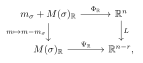
Comments
Corrections, questions, and mathematical discussion are welcome. Sign in with GitHub to comment. Comments are public.