There are some canonical choices of smooth flags in the toric setting.
Since $X$ is smooth and projective, we can choose a full-dimensional cone $\sigma $ in $\Sigma $ with rays $\rho _1,\ldots ,\rho _ n\in \sigma (1)$ such that $u_{\rho _1},\ldots ,u_{\rho _ n}$ form a basis of $N$. Define
Recall that $\Delta _{Y_{\bullet }}(L)\subseteq \mathbb {R}^ n$ is the Okounkov body defined in definition 19.4.8.
Proof.
We first reduce to the case where $D|_{U_{\sigma }}=0$. In fact, replacing $D$ by $D+\operatorname{div}\chi ^{m_{\sigma }}$ would result in changing $P_ D$ to $P_ D-m_{\sigma }$. So in view of (21.13.6), we may assume that $D|_{U_{\sigma }}=0$ and hence $m_{\sigma }=0$.
Fix $k\in \mathbb {Z}_{>0}$. Let $s\in \mathrm{H}^0(X,L^ k)$ be a non-zero toric eigen-section, say $\chi ^ m$ for some $m\in kP_ D\cap M$. The zero-divisor of $s$ on $U_{\sigma }$ is given by
\[ \sum _{i=1}^ n \langle m, u_{\rho _ i} \rangle D_{\rho _ i}, \]
\[ \nu _{Y_{\bullet }}(s)=\Bigl (\langle m, u_{\rho _1} \rangle ,\dots ,\langle m, u_{\rho _ n} \rangle \Bigr )=\Phi (m). \]
Conversely, every section of $L^ k$ is a finite linear combination of such characters. In the coordinates on $U_{\sigma }$ determined by $u_{\rho _1},\ldots ,u_{\rho _ n}$, the Okounkov valuation of a non-zero linear combination is the lexicographically first exponent among the characters with non-zero coefficient. Hence arbitrary sections give no valuations beyond the right-hand side of (21.13.34), and (21.13.34) follows.
$\square$
Example 21.13.35.74A6D2D50F46 Let us continue the example of $\mathbb {P}^2$ in example 21.13.12. We use the same notations. Take $\sigma _1$ as our reference cone, and $\rho _1=\sigma _5$, $\rho _2=\sigma _6$. Then
Example 21.13.36.BB6FCAD03597 Let us continue the example of $\mathrm{Bl}_{0}\mathbb {P}^2$ in example 21.13.15. This time, let us take $\sigma _1'$ as our reference cone and $\rho _1=\sigma _5$, $\rho _2=\sigma _7$. Then $Y_1$ is just the strict transform of the line $\{ [X_0:0:X_2]:X_0X_2\neq 0\} $ in $\mathbb {P}^2$, while $Y_2$ is the point $Y_1\cap E$, where $E$ is the exceptional divisor.
51BA09C1565221.13.37 The Okounkov body $\Delta _{Y_{\bullet }}(\mathrm{Bl}_{0}\mathbb {P}^2,\pi ^*\mathcal{O}_{\mathbb {P}^2}(1))$.
Note that it differs from the polytope in example 21.13.35.
Lemma 21.13.38.FCDBEF4DBD54 Let $\varphi \in \mathrm{PSH}_{\mathrm{tor}}(X,\theta )$ and assume that $\theta _{\varphi }$ is a Kähler current. Then $\varphi $ admits a quasi-equisingular approximation $(\varphi _ j)_ j$ with the following additional properties:
FE65BEEFF2E3
$\varphi _ j\in \mathrm{PSH}_{\mathrm{tor}}(X,\theta )$ and $\theta _{\varphi _ j}$ is a Kähler current for all $j\geq 1$;
5EC471277960
for each $j\geq 1$, there are $q_ j\in \mathbb Z_{>0}$ and toric eigen-sections
Proof.
Apply Demailly's Bergman-kernel approximation theorem [Theorem 13.21, Dem12] to the singular Hermitian metric $h\exp (-\varphi )$ on $L$. Since $\theta _{\varphi }$ is a Kähler current, the theorem applies to the Hilbert spaces
for $q\gg 1$, endowed with the $L^2$-norm induced by $h^ q\exp (-q\varphi )$ and a fixed Kähler volume form. The usual decreasing extraction in Demailly's construction gives a quasi-equisingular approximation; taking $q$ sufficiently large at each step ensures that the approximants still have Kähler Chern currents.
It remains to note that this construction is compatible with the torus action. Indeed, both $h$ and $\varphi $ are $T_ c$-invariant, hence the above Hilbert spaces and their $L^2$-inner products are $T_ c$-invariant. Since $T_ c$ is compact and abelian, each of these finite-dimensional Hilbert spaces admits an orthonormal basis consisting of toric eigen-sections. With such a basis, the corresponding Bergman potential has the displayed form and is $T_ c$-invariant. This proves the lemma.
$\square$
Theorem 21.13.39.8F3CCCDB83EC Let $\varphi \in \mathrm{PSH}_{\mathrm{tor}}(X,\theta )_{>0}$. Then
In particular, once $D$ is fixed, the Newton body $\Delta (\theta ,\varphi )$ depends only on the current $\theta _{\varphi }$, not on the specific choices of $h$, $\varphi $ and $s_ D$. It makes sense to write
A generalization of (21.13.41) to mixed volumes will be proved in theorem 21.13.84.
Proof.
We first reduce to the case where $D|_{U_{\sigma }}=0$. In fact, changing $D$ to $D+\operatorname{div}\chi ^{m_{\sigma }}$ would result in changing $F_{\theta }$ to $F_{\theta }-m_{\sigma }$. Hence, $F_{\varphi }$ changes to $F_{\varphi }-m_{\sigma }$. Therefore, $\Delta (\theta ,\varphi )$ becomes $\Delta (\theta ,\varphi )-m_{\sigma }$. Taking (21.13.6) into consideration, we may assume that $m_{\sigma }=0$.
Step 1. We first reduce to the case where $\theta _{\varphi }$ is a Kähler current.
By 13.13.47, we can find $\psi \in \mathrm{PSH}(X,\theta )$ such that $\psi \leq \varphi $ and $\theta _{\psi }$ is a Kähler current. Taking the average along $T_ c$, we may assume that $\psi $ is $T_ c$-invariant.
For each $t\in (0,1)$, we let
\[ \varphi _ t=(1-t)\psi +t\varphi . \]
Suppose that Kähler current case is known. Then we get
Comparing the volumes of both sides using proposition 21.13.28, (19.4.20), and the $\mathcal{I}$-goodness of toric singularities example 18.1.56, we find that
where $q\in \mathbb Z_{>0}$ and $s_1,\ldots ,s_ a\in \mathrm{H}^0(X,L^ q)$ are toric eigen-sections.
Let $m_1,\ldots ,m_ a\in qP_ D\cap M$ be the lattice points corresponding to $s_1,\ldots ,s_ a$.
Observe that
\[ \begin{aligned} \Delta (\theta ,\varphi ) =& \overline{\nabla F_{\varphi }(N_{\mathbb {R}})}\\ =& \left\{ m\in M_{\mathbb {R}} : F_{\varphi }(n)-\langle m,n \rangle \textup{ is bounded from below} \right\} \\ =& \left\{ m\in M_{\mathbb {R}}: q^{-1}\log \sum _{i=1}^ a \mathrm{e}^{\langle m_ i,n\rangle }-\langle m,n\rangle \textup{ is bounded below in } n \right\} \\ =& q^{-1}\mathrm{Conv}\{ m_1,\ldots ,m_ a\} , \end{aligned} \]
where we have applied (21.13.23) on the second line and 21.11.62 on the third line. Since $m_1,\ldots ,m_ a\in qP_ D$, the preceding formula also shows that
\[ \Delta (\theta ,\varphi )\subseteq P_ D. \]
Thus, if $m\in k\Delta (\theta ,\varphi )\cap M$, then $m\in kP_ D\cap M$, and $\chi ^ m$ indeed determines a global section of $L^ k$.
In particular, by the same separation argument as in 21.11.60, for any $k\in \mathbb {Z}_{>0}$ and any $m\in k\Delta (\theta ,\varphi )\cap M$, we have
\[ |\chi ^ m|^2 \mathrm{e}^{-k\varphi } \]
is bounded from above on $T(\mathbb {C})$. In other words, the section $s$ of $L^ k$ corresponding to $m$ satisfies
Comparing the volumes of both sides using proposition 21.13.28 and (19.4.20), we conclude that the equality holds and (21.13.40) follows.
$\square$
The following two consequences are both due to Yi Yao.
Corollary 21.13.42.B202075FB15E Let $E$ be a $T$-invariant prime divisor on $X$ corresponding to a ray $\rho \in \Sigma (1)$. Then for any $\varphi \in \mathrm{PSH}_{\mathrm{tor}}(X,\theta )_{>0}$, we have
Proof.
This follows immediately from theorem 21.13.39 and theorem 19.4.51. In fact, since $X$ is projective and smooth, there is always a $T$-invariant smooth flag $Y_{\bullet }$ with $Y_1=E$.
$\square$
This result seems new even in the ample setting. Intuitively, after taking theorem 21.13.45 into consideration as well, in the ample case the generic Lelong number $\nu (\varphi ,E)$ is the rescaled “distance” from $\Delta (\theta ,\varphi )$ to the facet of $P_ D$ corresponding to $E$.2
Corollary 21.13.43.C521E79AA7F6 Let $Y\subseteq X$ be a $T$-invariant subvariety corresponding to a cone $\sigma $ in $\Sigma $, and let $\varphi \in \mathrm{PSH}_{\mathrm{tor}}(X,\theta )_{>0}$. Then the following are equivalent:
29543A48DCD3
$\nu (\varphi ,Y)=0$;
132682CA7C05
there is a point $m\in \Delta (\theta ,\varphi )$ such that $\langle m-m_{\rho },u_{\rho }\rangle =0$ for any $\rho \in \sigma (1)$;
Recall that $Q_{\sigma }$ is defined in (21.13.7).
Proof.2 $\iff $ 3. This follows from the definition of $Q_{\sigma }$ in (21.13.7).
1 $\iff $ 2. Let $\rho _1,\ldots ,\rho _ r$ be the rays of $\sigma $. Up to replacing $D$ by a translation, we may assume that $m_{\sigma }=0$. Hence, we may take $m_{\rho _ i}=0$ for all $i$.
Let $\pi \colon Z\rightarrow X$ be the blow-up of $X$ along $Y$. See [Page 132, CLS11] for the basic properties of the toric blow-up. Take the divisor $\pi ^*D$ on $Z$. We choose the pull-back metric $\pi ^*h$ on $\pi ^*L$. Then $F_{\pi ^*\theta }$ can be taken as $\pi ^*F_{\theta }$ by (21.13.23). It follows that $\Delta (\theta ,\varphi )=\Delta (\pi ^*\theta ,\pi ^*\varphi )$. On the other hand, the ray corresponding to the exceptional divisor $E$ is generated by $u_{\rho _1}+\cdots +u_{\rho _ r}$. Since $X$ is smooth, this vector is primitive.
Recall that the support function of $\pi ^*D$ is the same as the support function of $D$, see [Proposition 6.2.7, CLS11]. In particular, we can take the Cartier datum $m_{\rho }=m_{\sigma } \mod M(\rho )$, where $\rho $ is the ray corresponding to $E$.
where we applied proposition 21.13.33 in the last equality. Therefore, (21.13.49) follows. In particular, (21.13.47) follows from proposition 21.13.28.
Next we prove (21.13.48). Take a smooth function $\chi \colon N_{\mathbb {R}}\rightarrow [0,1]$ so that
37909700D0C1
$\operatorname{Supp}\chi $ is compact;
C1605365568C
$\chi \equiv 1$ on a neighbourhood of $0$.
Fix a $T_ c$-invariant volume form $\mu $ on $T(\mathbb {C})$. Then $(\operatorname{Trop}^*\chi )\mu $ can be regarded as a $T_ c$-invariant smooth non-negative measure on $X$. After choosing a suitable normalizing constant $C>0$, there is a unique solution
This is proved in [Theorem B, BEGZ10]. The uniqueness of $\varphi $ further guarantees its $T_ c$-invariance. Since $\varphi $ has minimal singularities, $F_{\varphi }\sim F_{V_{\theta }}$. Next, using proposition 21.13.28, the Monge–Ampère equation (21.13.50) implies
It follows from the regularity theorem [Theorem 2.19, BB13] and (21.13.49) that $F_{\varphi }\sim \operatorname{Supp}_{P_ D}$. Hence, (21.13.48) follows.
$\square$
As an interesting consequence of (21.13.51), we have a geometric description of the divisorial Zariski decomposition in the toric setting: The negative part of $D$ is given by
 Pome
Pome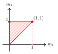
Comments
Corrections, questions, and mathematical discussion are welcome. Sign in with GitHub to comment. Comments are public.