19.5 Transcendental partial Okounkov bodiesA2D41AECAD65

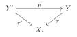
Proof. Take another map $\pi '\colon Y'\rightarrow X$ with the same properties. We want to show that $\pi $ and $\pi '$ define the same $\Delta _{Y_{\bullet }}(T)$. We may assume that $\pi '$ dominates $\pi $ through $p\colon Y'\rightarrow Y$, so that we have a commutative diagram

We take $D$ and $R$ as in (19.5.8). Then

Write $(Z_{\bullet },g)$ and $(Z_{\bullet }',g')$ for the liftings of $Y_{\bullet }$ to $Y$ and $Y'$ respectively. We need to prove that

By theorem 19.5.4, applied to the class $\{ R\} $, we have

By proposition 19.3.14, applied to the divisor current $[D]$, we also have

Finally, proposition 19.3.17 gives

Multiplying by $(g')^{-1}$ gives the desired equality. $\square$

Proof. We first show that

Using 19.5.11, we may assume that $T$ and $S$ have log singularities along effective $\mathbb {Q}$-divisors $E$ and $F$ respectively. By assumption, $E\geq F$. Replacing $T$ and $S$ by $T-[F]$ and $S-[F]$ respectively, we may assume that $F=0$, cf. (19.5.9).

In this case, we need to show that

which is obvious.

Next we prove that

By 19.5.11 and theorem 19.5.4 again, we may assume that $T$ has log singularities. We take $D$ and $R$ as in (19.5.8). We need to show that

which is again obvious.

Finally, (19.5.13) follows immediately from theorem 19.5.4. $\square$

Proof. It is more convenient to use the language of $\theta $-psh functions at this point. Let $\psi _ k$ (resp. $\varphi _ k$) denote the potentials in $\mathrm{PSH}(X,\theta )$ corresponding to $S_ k$ (resp. $T_ k$) for each $k\geq 1$. Note that $\psi _ k$ and $\varphi _ k$ are unique up to additive constants. By proposition 5.18.12, for any small rational $\epsilon >0$, $j>0$, we can find $k>0$ so that

By 19.5.12,

On the other hand, observe that

In fact, the $\supseteq $ direction follows from 19.5.12, so it suffices to show that the two sides have the same volume, which follows from (19.5.13).

It follows that

The other inclusion follows by symmetry. $\square$

Proof. Take a quasi-equisingular approximation $(T_ j)_ j$ of $T$ in $\mathcal{Z}_+(X,\alpha )$. Note that $\Delta _{Y_{\bullet }}(T_ j)$ is decreasing in $j$, as follows from 19.5.12. Our assertion follows from (19.5.13) and theorem 16.9.57. $\square$

Proof. We first prove (19.5.21). Taking quasi-equisingular approximations, we reduce immediately to the case where $T$ has analytic singularities. By 19.5.11, we may assume that $T$ has log singularities. Take $D$ and $R$ as in (19.5.8). By definition again, it suffices to show that

which is clear by definition.

Next we prove (19.5.22). Thanks to (19.5.21), it remains to prove that both sides have the same volume:

This is proved in proposition 18.1.27. $\square$

Proof. 1 By (19.5.25) and (19.5.19), for any Kähler form $\omega $ on $X$,

The right-hand side is computed in proposition 18.1.27. Hence, (19.5.27) follows.

2 Fix a Kähler form $\omega $ on $X$. By corollary 19.5.17, for each $j\geq 1$,

It remains to show that

The $\subseteq $ direction is clear. Comparing the volumes using theorem 19.5.4, we conclude that equality holds.

3 This follows from 1 and 2.

4 Let $(T_ j)_ j$ be a sequence in $\mathcal{Z}_+(X,\alpha )_{>0}$ converging to $T\in \mathcal{Z}_+(X,\alpha )_{>0}$ with respect to $d_ S$. We want to show that $\Delta _{Y_{\bullet }}(T_ j)\xrightarrow {d_{\mathrm{Haus}}} \Delta _{Y_{\bullet }}(T)$. By 2, replacing the potential of each current by its $\mathcal I$-model representative does not change its partial Okounkov body. Thus we may represent the singularity types by model potentials of uniformly positive mass. Applying proposition 16.9.17, after passing to a subsequence we may sandwich the sequence between an increasing and a decreasing sequence converging to $T$ in $d_ S$. Hence it suffices to treat the monotone cases.

In either monotone case, 2 gives monotonicity of the convex bodies, while 1 and corollary 16.9.13 give convergence of their volumes to $\operatorname{vol}\Delta _{Y_{\bullet }}(T)$. Every Hausdorff cluster point is therefore a monotone limit with the same volume as $\Delta _{Y_{\bullet }}(T)$, hence is equal to $\Delta _{Y_{\bullet }}(T)$.

5 We may assume that $T$ is $\mathcal{I}$-good. It follows from 4 and theorem 18.1.2 that we may reduce to the case where $T$ has analytic singularities. Our assertion follows from 19.5.11.

6 By (19.5.25), in order to prove (19.5.28), we may assume that $T$ and $S$ are both Kähler currents. Take quasi-equisingular approximations $(T_ j)_ j$ and $(S_ j)_ j$ of $T$ and $S$ respectively. By theorem 16.9.45, $T_ j+S_ j\xrightarrow {d_ S} T+S$. By 4, we may therefore assume that $T$ and $S$ have analytic singularities. Replacing $X$ by a suitable modification, we may assume that $T$ and $S$ both have log singularities, say

where $D$ and $D'$ are $\mathbb {Q}$-divisors on $X$ and $R$ and $R'$ are closed positive $(1,1)$-currents with bounded potentials. We need to show that

By proposition 19.3.9, this is equivalent to

which is already proved in theorem 19.5.4. $\square$

Proof. We may assume that $\mathrm{dd}^{\mathrm{c}}h$ has positive mass and is $\mathcal{I}$-good. By the $d_ S$-continuity of both sides of (19.5.30) as proved in theorem 19.5.26 and theorem 19.4.30, together with theorem 18.1.2, we may assume that $\mathrm{dd}^{\mathrm{c}}h$ has analytic singularities.

In this case, using the birational invariance of both sides of (19.5.30) as proved in proposition 19.4.32 and theorem 19.5.26, we may assume that $\mathrm{dd}^{\mathrm{c}}h$ has log singularities. Finally, after all these reductions, the equality (19.5.30) holds by construction. $\square$

Proof. Step 1. We first reduce to the case where $\beta $ is a Kähler class.

Take a Kähler class $\alpha $ on $X$. It follows from the volume formula in theorem 19.5.4 that

Since $\beta |_{Y_1}$ is nef, hence pseudo-effective, definition 19.5.24 similarly gives

So it suffices to prove (19.5.33) with $\beta +\epsilon \alpha $ in place of $\beta $.

Step 2. Assume that $\beta $ is a Kähler class. The $\supseteq $ direction in (19.5.33) follows from the extension theorem theorem 5.18.18. To prove the other direction, recall that by theorem 19.5.4, for $t>0$ small enough, we have

As $t\to 0+$, the right-hand side converges to $\Delta _{Y_1\supseteq \cdots \supseteq Y_ n}(\beta |_{Y_1})$ with respect to the Hausdorff metric as a consequence of theorem 19.5.4, while the left-hand side converges to

by 19.7.9. We conclude our assertion. $\square$

Proof. Let $\omega $ be a Kähler form on $X$. The last assertion follows from the first by perturbing $\theta $ to $\theta +\epsilon \omega $.

Step 1. We first handle the case where $T$ has analytic singularities. Let $\pi \colon Z\rightarrow X$ be a modification such that

1. 90254E23C2B2

   $Y_{\bullet }$ admits a lifting $(W_{\bullet },g)$, and

2. CA8486D14D75

   $\pi ^*T=[D]+R$, where $D$ is an effective $\mathbb {Q}$-divisor on $Z$ and $R$ is a closed positive $(1,1)$-current with bounded potential.

This is possible by theorem 5.18.8 and theorem 19.3.19.

By 20.2.24,

where $\Pi \colon W_1\rightarrow Y_1$ is the restriction of $\pi $. It follows from theorem 19.5.26 that

Taking (19.3.13) into account, we find that it suffices to show that

We may assume that $\pi $ is the identity map. Since $\nu (T,Y_1)=0$, the divisor $D$ does not contain $Y_1$. Hence we have

Note that $[D]|_{Y_1}$ is the current of integration along an effective $\mathbb {Q}$-divisor on $Y_1$.

In particular,

The first coordinate of $\nu _{Y_{\bullet }}([D])$ is $0$, and the remaining coordinates are exactly $\nu _{Y_1\supseteq \cdots \supseteq Y_ n}([D]|_{Y_1})$. Thus it suffices to show that

Since $R$ has bounded potential, its cohomology class is nef; it is big because $T$ is a Kähler current. Thus the last identity is exactly 19.5.32.

Step 2. Next we consider the case where $T$ is a Kähler current. Take a quasi-equisingular approximation $(T_ j)_ j$ of $T$ in $\mathcal{Z}_+(X,\alpha )$. From Step 1, we know that for large $j\geq 1$,

Letting $j\to \infty $ and applying theorem 19.5.26 and proposition 20.2.22, we conclude (19.5.35). $\square$

Proof. We argue by induction on $n\geq 0$. The case $n=0$ is of course trivial. Let us assume that $n>0$ and the case $n-1$ has been proved.

We first observe that by theorem 19.5.26,

By proposition 18.1.27 5, removing the divisorial part does not change the volume. Comparing the volumes of both sides using theorem 19.5.26 and proposition 18.1.27, we find that equality holds:

Replacing $T$ by $T-\nu (T,Y_1)[Y_1]$, we may therefore assume that $\nu (T,Y_1)=0$. It suffices to apply 19.5.34 and the inductive hypothesis. $\square$

Proof. When $T$ is a Kähler current, this follows from theorem 19.5.37.

In general, by definition, $\nu _{Y_{\bullet }}(T)=\nu _{Y_{\bullet }}(T+\omega )$ for any Kähler form $\omega $ on $X$. It follows that

for any Kähler form $\omega $. It follows that $\nu _{Y_{\bullet }}(T)\in \Delta _{Y_{\bullet }}(T)$. $\square$

Proof. The $\supseteq $ direction in (19.5.41) follows from corollary 19.5.39 together with theorem 19.5.26 2.

Let us write

for the time being.

Step 1. Assume that $T$ has analytic singularities. We have

It follows easily from theorem 19.5.4 that the volume of the right-hand side is equal to the volume of $\Delta _{Y_{\bullet }}(T)$, so (19.5.41) holds.

Step 2. Assume that $T$ is a Kähler current. Take a quasi-equisingular approximation $T_ j\in \mathcal{Z}_+(X,\alpha )$ of $T$. Next we use the language of psh functions. Let $\varphi _ j,\varphi \in \mathrm{PSH}(X,\theta )$ be the potentials corresponding to $T_ j,T$ for each $j\geq 1$.

Fix an integer $N>0$. For large enough $j\geq 1$, we can find $\psi _ j\in \mathrm{PSH}(X,\theta )_{>0}$ such that

The existence of $\psi _ j$ follows from 13.13.30. It follows that

We claim that

Let $x$ be a point in the right-hand side. Fix $N>0$. For all large $j$, choose

with $y_ j\to x$. By the preceding inclusion,

The points $x,y_ j,z_ j$ all lie in the compact set $\Delta _{Y_{\bullet }}(\alpha )$ after taking closures, by corollary 19.5.39. Hence, letting $j\to \infty $ and then $N\to \infty $, we get $x\in \overline{D_{Y_{\bullet }}(T)}$, proving the claim. Therefore, by Step 1, we conclude that

The reverse direction is already known.

Step 3. Finally, consider the general case. Take a Kähler current $T'\in \mathcal{Z}_+(X,\alpha )$ more singular than $T$ (the existence of which is given by 13.13.47). For each $\epsilon \in (0,1)$, we know that

Letting $\epsilon \to 0+$ and using the $d_ S$-continuity in theorem 19.5.26 4, we find that

As the other inclusion is already known, we conclude. $\square$

Proof. By theorem 19.5.40, it is clear that

On the other hand, we clearly have

for any Kähler form $\omega $ on $X$. It follows that

By theorem 19.5.37, the right-hand side is just $\nu _{Y_{\bullet }}(T+\omega )=\nu _{Y_{\bullet }}(T)$. We conclude the proof. $\square$