The set $\mathcal{P}(N_{\mathbb {R}},P_ D)$ is defined in definition 21.11.41. As before, we write $F_{\varphi }$, $G_{\varphi }$ for the functions determined by this construction.
Proof.
The proof is similar to that of theorem 21.12.13, but due to its importance, we give the details. Again, the correspondence between 2 and 3 follows easily from proposition 21.11.38.
Given $\varphi $, we can construct $F_{\varphi }$ in 2 as explained earlier in (21.13.26). Conversely, suppose that $F\in \mathcal{P}(N_{\mathbb {R}},P_ D)$, then $F\preceq F_{V_{\theta }}$ by theorem 21.13.45. Then
by 21.12.7. Since $F\preceq F_{V_{\theta }}$, we see that $\operatorname{Trop}^*(F-F_{\theta })$ is bounded from above. It follows that Grauert–Remmert's extension theorem theorem 5.14.10 is applicable, and this function extends to a unique $\theta $-psh function $\varphi $. The uniqueness of the extension guarantees that $\varphi \in \mathrm{PSH}_{\mathrm{tor}}(X,\theta )$.
The two maps are inverse to each other by construction.
$\square$
We fix a model potential $\phi \in \mathrm{PSH}_{\mathrm{tor}}(X,\theta )_{>0}$ with Newton body $\Delta (\theta ,\phi )$.
A similar argument guarantees the following:
Corollary 21.13.54.1D4A688AAB93 There is a canonical bijection between the following sets:
0180BB40C5AC
The set of $\varphi \in \mathrm{PSH}_{\mathrm{tor}}(X,\theta ;\phi )$,
C7ECD31C42B2
the set of $F\in \mathcal{P}(N_{\mathbb {R}},\Delta (\theta ,\phi ))$, and
5661D01495BD
the set of closed proper convex functions $G\in \mathrm{Conv}(M_{\mathbb {R}})$ satisfying
Proposition 21.13.57.BC781EB76285 Let $(\varphi _ i)_{i\in I}$ be a family in $\mathrm{PSH}_{\mathrm{tor}}(X,\theta )$ uniformly bounded from above. Then $\operatorname *{sup}_{i\in I}{}\! {}^{*} \varphi _ i\in \mathrm{PSH}_{\mathrm{tor}}(X,\theta )$ and
Similarly, if $\{ \varphi _ i\} _{i\in I}$ is a decreasing net in $\mathrm{PSH}_{\mathrm{tor}}(X,\theta )$ such that $\inf _{i\in I}\varphi _ i\not\equiv -\infty $, then $\inf _{i\in I}\varphi _ i\in \mathrm{PSH}_{\mathrm{tor}}(X,\theta )$ and
Proposition 21.13.58.0728D8B152D3 Let $\varphi \in \mathrm{PSH}_{\mathrm{tor}}(X,\theta )$. Then $P_{\theta }[\varphi ]\in \mathrm{PSH}_{\mathrm{tor}}(X,\theta )$ and
Hence $P_{\theta }[\varphi ]\in \mathrm{PSH}_{\mathrm{tor}}(X,\theta )$ by proposition 21.13.55, proposition 21.13.56, proposition 21.13.57. The same results give
If $x\in \operatorname{Dom}G_{\varphi }$, then $G_{\varphi }(x)-C\leq G_{V_{\theta }}(x)$ for all large enough $C$, so $K(x)=G_{V_{\theta }}(x)$. If $x\notin \operatorname{Dom}G_{\varphi }$, then $K(x)=\infty $. By proposition 21.11.34, we have $\Delta (\theta ,\varphi )=\overline{\operatorname{Dom}G_{\varphi }}$. Moreover, theorem 21.13.45 gives $F_{V_{\theta }}\sim \operatorname{Supp}_{P_ D}$, hence $G_{V_{\theta }}\sim \chi _{P_ D}$ by Legendre duality. In particular, $G_{V_{\theta }}$ is finite and continuous on $P_ D$. Thus the lower semicontinuous regularization of $K$ is equal to $G_{V_{\theta }}$ on $\Delta (\theta ,\varphi )$ and equal to $\infty $ outside $\Delta (\theta ,\varphi )$.
$\square$
As a consequence, we have
Corollary 21.13.60.396E3B9D09BD Let $\varphi ,\psi \in \mathrm{PSH}_{\mathrm{tor}}(X,\theta )$. Then the following are equivalent:
Proof.1 $\iff $ 2. This follows from the $\mathcal{I}$-goodness of $\varphi $ and $\psi $, see example 18.1.56.
1 $\iff $ 3. When $\varphi ,\psi \in \mathrm{PSH}_{\mathrm{tor}}(X,\theta )_{>0}$, this follows from proposition 21.13.58.
In general, fix an ample toric-invariant divisor $H$ on $X$ and a toric-invariant Hermitian metric $h_ H$ on $\mathcal{O}_ X(H)$ such that $\omega _ H\coloneqq \mathrm{dd}^{\mathrm{c}}h_ H$ is a Kähler form. We perturb $L$ to $L+m^{-1}H$ for $m\in \mathbb {Z}_{>0}$, then thanks to 21.11.47, we find that
\[ \mathrm{PSH}_{\mathrm{tor}}(X,\theta )/\sim _{\mathcal{I}}\rightarrow \left\{ K\in \mathcal{K}_ n: K \subseteq P_ D \right\} \]
is well-defined and injective.
In order to see the surjectivity, take $K\in \mathcal{K}_ n$, $K\subseteq P_ D$. Let $\chi _ K$ be the characteristic function of $K$ as defined in example 21.11.5. Since $\chi _ K$ satisfies Condition 3 of theorem 21.13.53, we can find $\varphi \in \mathrm{PSH}_{\mathrm{tor}}(X,\theta )$ so that $\chi _ K=G_{\varphi }$. Then $\Delta (\theta ,\varphi )=K$ due to proposition 21.11.34.
$\square$
Next we handle subgeodesics.
Proposition 21.13.62.D5C47A3AE82D Let $\varphi _0,\varphi _1\in \mathrm{PSH}_{\mathrm{tor}}(X,\theta )$. There is a canonical bijection between the following sets:
7620AF887D78
The set of $T_ c$-invariant subgeodesics from $\varphi _0$ to $\varphi _1$;
E254BA3D3052
the set of convex functions $F\colon N_{\mathbb {R}}\times (0,1)\rightarrow \mathbb {R}$ such that for each $r\in (0,1)$, the function
Proof.
We begin with a subgeodesic $(\varphi _ t)_{t\in (0,1)}$ from $\varphi _0$ to $\varphi _1$. Then we define $F\colon N_{\mathbb {R}}\times (0,1)\rightarrow \mathbb {R}$ as follows:
Let $t_ j\to 0+$. Since $\varphi _{t_ j}\to \varphi _0$ in $L^1$, after passing to a subsequence we have almost-everywhere convergence on $X$. Restricted to the open torus and using the tropical coordinates, this gives $F_{t_ j}\to F_{\varphi _0}$ almost everywhere on $N_{\mathbb R}$. Since the $F_{t_ j}$'s are convex and locally uniformly bounded above, theorem 21.11.20 upgrades this to pointwise convergence everywhere. As the limit is independent of the subsequence, $F_ t\to F_{\varphi _0}$ everywhere as $t\to 0+$. Similarly, $F_ t\to F_{\varphi _1}$ everywhere as $t\to 1-$.
Next we show that $F$ is convex. Let $p_1\colon X\times S\rightarrow X$ be the projection, where
is plurisubharmonic and $T_ c\times S^1$-invariant. Fix a small enough $\epsilon >0$. We can find a decreasing sequence of $T_ c\times S^1$-invariant plurisubharmonic functions $\Psi _ i$ on $T(\mathbb {C})\times S_{\epsilon }$ converging to $\Psi $ everywhere, where
for some $F_ i\colon N_{\mathbb {R}}\times (\epsilon ,1-\epsilon )\rightarrow \mathbb {R}$.
The same computation as in 21.12.7 shows that $F_ i$ is convex. It follows that $F$, as the decreasing limit of $F_ i$, is also convex on $N_{\mathbb {R}}\times (\epsilon ,1-\epsilon )$. Since $\epsilon >0$ is arbitrary, we conclude that $F$ is convex on $N_{\mathbb {R}}\times (0,1)$.
Conversely, suppose that we are given $F$ in 2. We define $\Phi \colon T(\mathbb {C})\times S\rightarrow \mathbb {R}$ using (21.13.64). The arguments in the previous part can be reversed to show that $\Phi $ is $p_1^*\theta |_{T(\mathbb {C})\times S}$-psh.
for some constant $C\in \mathbb {R}$ independent of the choice of $t$. Therefore, $\Phi $ is bounded from above and hence, by theorem 5.14.10, admits a unique $p_1^*\theta $-psh extension to $X\times S$, which we still denote by $\Phi $. We let
\[ \varphi _ t(x)=\Phi (x,\mathrm{e}^{-t/2}) \]
for all $t\in (0,1)$ and $x\in X$. We claim that $(\varphi _ t)$ is a subgeodesic from $\varphi _0$ to $\varphi _1$.
For this purpose, we only need to show that $(\varphi _ t)_{t\in (0,1)}$ has the correct boundary value. But from our assumption in 2, we know that as $t\to 0+$ (resp. $t\to 1-$), $\varphi _ t\to \varphi _0$ (resp. $\varphi _ t\to \varphi _1$) almost everywhere. In particular, $\sup _ X \varphi _ t\geq -C'$ for some large constant $C'>0$ independent of $t\in (0,1)$. Therefore, together with (21.13.65), we deduce from proposition 5.17.3 that $\{ \varphi _ t\} _{t\in (0,1)}$ is a relatively compact family with respect to the $L^1$-topology. We need to show that each cluster point $\psi $ as $t\to 0+$ is equal to $\varphi _0$. But we already know that $\psi =\varphi _0$ almost everywhere. Hence we deduce $\psi =\varphi _0$ from proposition 5.14.6. As $t\to 0+$, we have $\varphi _ t\xrightarrow {L^1}\varphi _0$. Similarly, as $t\to 1-$, we have $\varphi _ t\xrightarrow {L^1}\varphi _1$.
The two constructions are inverse to each other by construction.
$\square$
Corollary 21.13.66.03A225BFC03C Let $\varphi _0,\varphi _1\in \mathrm{PSH}_{\mathrm{tor}}(X,\theta )$. Then there is a canonical bijection between the following sets:
3A549D6065ED
The set of $T_ c$-invariant subgeodesics from $\psi _0$ to $\psi _1$, where $\psi _0,\psi _1\in \mathrm{PSH}_{\mathrm{tor}}(X,\theta )$ and $\psi _0\leq \varphi _0$, $\psi _1\leq \varphi _1$;
C3D9271539D5
the set of closed proper convex functions $\Psi $ on $M_{\mathbb {R}}\times \mathbb {R}$ such that there is a closed proper convex function $G\in \mathrm{Conv}(M_{\mathbb {R}})$ satisfying
for all $m\in M_{\mathbb {R}}$ and $s\in \mathbb {R}$.
Proof.
Let us begin with a subgeodesic $(\psi _ t)_{t\in (0,1)}$ as in 1. Let $F$ be the convex function as in proposition 21.13.62. We extend $F$ to a function $F\colon N_{\mathbb {R}}\times \mathbb {R}\rightarrow \mathbb {R}$ as follows: For any $n\in N_{\mathbb {R}}$, we define
Then $F$ is a proper closed convex function on $N_{\mathbb {R}}\times \mathbb {R}$. Let $\Psi $ be the Legendre transform of $F$. Then $\Psi $ is a proper closed convex function on $M_{\mathbb {R}}\times \mathbb {R}$ by theorem 21.11.24. By (21.11.23), for any $m\in M_{\mathbb {R}}$ and $s\in \mathbb {R}$, we have
Conversely, let us begin with a function $\Psi $ as in 2. Let $F$ be the Legendre transform of $\Psi $. We first observe that $F(n,t)=\infty $ for all $n\in N_{\mathbb {R}}$ and $t\not\in [0,1]$. Indeed, the upper bound $\Psi \leq G+(s\lor 0)$ gives
The estimates above give $F_0\leq F_{\varphi _0}$ and $F_1\leq F_{\varphi _1}$, and also show that $F_0,F_1\in \mathcal{P}(N_{\mathbb {R}},P_ D)$. Let $\psi _0,\psi _1\in \mathrm{PSH}_{\mathrm{tor}}(X,\theta )$ be the corresponding potentials given by theorem 21.13.53. Then $\psi _0\leq \varphi _0$ and $\psi _1\leq \varphi _1$. Applying proposition 21.13.62 to the restriction of $F$ to $N_{\mathbb {R}}\times (0,1)$, we get a subgeodesic $(\psi _ t)_{t\in (0,1)}$ from $\psi _0$ to $\psi _1$. Thus $(\psi _ t)_{t\in (0,1)}$ satisfies 1. The two operations are inverse to each other by construction.
$\square$
As an immediate corollary,
Corollary 21.13.68.551D529C92A2 Let $\varphi _0,\varphi _1\in \mathrm{PSH}_{\mathrm{tor}}(X,\theta )\cap \mathrm{PSH}(X,\theta )_{>0}$. Then the following are equivalent:
8E1A729499A6
$\varphi _0\sim _ P \varphi _1$;
39AFF113945C
there is a subgeodesic from $\varphi _0$ to $\varphi _1$.
If these conditions are satisfied, let $(\varphi _ t)_{t\in (0,1)}$ be the geodesic from $\varphi _0$ to $\varphi _1$. Then $\varphi _ t\in \mathrm{PSH}_{\mathrm{tor}}(X,\theta )$ for all $t\in (0,1)$ and
Proof.
The equivalence between 1 and 2 follows from a general fact theorem 16.8.32. In the toric case, 2 $\implies $ 1 can also be argued more directly.
Assume that these conditions are satisfied. Let $(\varphi _ t)_{t\in (0,1)}$ be the geodesic from $\varphi _0$ to $\varphi _1$. Since the geodesic is the upper envelope of toric subgeodesics, $\varphi _ t\in \mathrm{PSH}_{\mathrm{tor}}(X,\theta )$ for all $t\in (0,1)$. Let $\Psi '$ be the proper convex function on $M_{\mathbb {R}}\times \mathbb {R}$ defined by corollary 21.13.66. Then $\Psi '$ is the minimum of all $\Psi $ satisfying (21.13.67). We claim that
It suffices to show that the right-hand side is proper, namely, $G_{\varphi _0}\lor G_{\varphi _1}$ is not identically $\infty $. But recall that by proposition 17.10.7, we have $\varphi _0\land \varphi _1\in \mathrm{PSH}(X,\theta )$. Therefore, by proposition 21.13.56,
Proof.
First observe that given $g$ as in 2, (21.13.72) indeed induces a geodesic ray in $\mathcal{R}_{\mathrm{tor}}(X,\theta ;\phi )$ thanks to corollary 21.13.68. Therefore, we have a map from 2 to 1.
Conversely, given $\ell \in \mathcal{R}_{\mathrm{tor}}(X,\theta ;\phi )$, it follows from corollary 21.13.68 that $G_{\ell _ t}$ is linear in $t\geq 0$ after restriction to $\operatorname{Int}\{ G_{\phi }<\infty \} $. Let
Hence, $g'$ is a proper convex function on $M_{\mathbb {R}}$. Define $g=\operatorname{cl}g'$. Then $g$ is a proper closed convex function on $M_{\mathbb {R}}$, and $\overline{\operatorname{Dom}g}=\Delta (\theta ,\phi )$. We have therefore a map from 1 to 2.
It remains to argue that this map is the converse of the preceding map from 2 to 1. The non-trivial point is to verify (21.13.72) holds for the $g$ we just constructed. Fix $t>0$. We need to show that
\[ G_{\ell _ t}=G_{\phi }+tg. \]
This holds on $\operatorname{Int}\{ G_{\phi }<\infty \} $ by corollary 21.13.68 and the definition of $g$, but then it holds everywhere thanks to proposition 21.11.18. Our assertion follows.
$\square$
In particular, we can make the corresponding test curve more explicit.
Corollary 21.13.73.AFC1919DC91A Let $\ell \in \mathcal{R}_{\mathrm{tor}}(X,\theta ;\phi )$ and $g$ be the function as in corollary 21.13.71. Then
Next we consider the trace operator studied in section 20.2. We wish to understand the trace operator in the toric situation. For this purpose, we will need to fix a $T$-invariant subvariety $Y\subseteq X$. Let $\sigma $ be the corresponding cone in $\Sigma $, and let $Q_{\sigma }\subseteq P_ D$ be the subset defined in (21.13.7). The cocharacter lattice of $Y$ is given by
where $\langle \sigma \rangle $ is the linear span of $\sigma $. See [(3.2.6), CLS11]. In particular, we have a canonical identification of the character lattice $M(\sigma )$ of $Y$:
\[ M(\sigma )=\sigma ^{\perp }\cap M, \]
which is compatible with our previous notation (21.13.3). Let $i_{\sigma }\colon M(\sigma )\rightarrow M$ be the inclusion map. Let $T_ Y$ be the torus of $Y$. Then we have a natural surjection $q_ T\colon T\rightarrow T_ Y$. In particular, the tropicalization map
Choose a representative $m_{\sigma }\in M$ of the Cartier datum along $\sigma $. Then $m-m_{\sigma }\in M(\sigma )_{\mathbb {R}}$ for every $m\in Q_{\sigma }$. We let
where $\rho \not\preceq \sigma $ means that $\rho $ is not a face of $\sigma $. Then $\mathcal{O}_ Y(D_ Y)=L|_ Y$. Equivalently, $D_ Y$ is the divisor associated to the rational section
\[ s_{D_ Y}\coloneqq (\chi ^{m_{\sigma }}s_ D)|_ Y \]
of $L|_ Y$. Write $P_{D_ Y}$ for the polytope of $D_ Y$. With this choice, $Q_{\sigma }-m_{\sigma }$ is naturally contained in $P_{D_ Y}$.
Theorem 21.13.75.0BA5B8CFD15F With the above choice of representative $m_{\sigma }$, let $\varphi \in \mathrm{PSH}_{\mathrm{tor}}(X,\theta )_{>0}$ satisfy $\nu (\varphi ,Y)=0$. If $\operatorname{Tr}_ Y^{\theta }(\varphi )$ is defined and $\operatorname{vol}(\theta |_ Y,\operatorname{Tr}_ Y^{\theta }(\varphi ))>0$5, then
Observe that the condition $\nu (\varphi ,Y)=0$ means exactly that $\Delta (\theta ,\varphi )\cap Q_{\sigma }\neq \varnothing $ by corollary 21.13.43.
Since $Y$ itself is a smooth toric variety, the preceding constructions of $X$ all apply to $Y$. We briefly summarize the situation in 21.13.76.
Notions for $X$
Notions for $Y$
$N$
$N(\sigma )$
$M$
$M(\sigma )$
$\Sigma $
$\mathrm{Star}(\sigma )$
$D$
$D_ Y$
$L$
$L|_ Y$
$h$
$h|_ Y$
$\theta $
$\theta |_ Y$
$\operatorname{Trop}$
$\operatorname{Trop}_ Y$
$P_ D$
$P_{D_ Y}$
$s_ D$
$s_{D_ Y}$
9C7AF9D665D821.13.76 The correspondence between $X$ and $Y$
Recall that $\mathrm{Star}(\sigma )$ is the fan in $N(\sigma )_{\mathbb {R}}$ consisting of $\bar{\tau }$ for all faces $\tau \in \Sigma $ containing $\sigma $, where $\bar{\tau }$ is the image of $\tau $ in $N(\sigma )_{\mathbb {R}}$. See [Proposition 3.2.7, CLS11].
Proof.
The idea of the proof is that since 19.5.34, 19.5.36 describe how partial Okounkov bodies behave under restriction, and theorem 21.13.39 compares partial Okounkov bodies with Newton bodies, we can deduce the behavior of Newton bodies under restriction as well.
First we note that by our assumption, $L|_ Y$ is a big line bundle. In particular, if we set $r=\dim \sigma $, then $\dim Y=n-r$.
We also note that $\operatorname{Tr}_ Y^\theta (\varphi )$ is $T_{Y,c}$-invariant. Indeed, for any $g\in T_ c$, let $g_ Y$ be the induced automorphism of $Y$. Then $g_ Y^*\operatorname{Tr}_ Y(\varphi )$ is again a trace of $g^*\varphi =\varphi $ along $Y$. Hence $g_ Y^*\operatorname{Tr}_ Y(\varphi )\sim _ P\operatorname{Tr}_ Y(\varphi )$ by proposition 20.2.8. Since $\theta |_ Y$ is $T_{Y,c}$-invariant and the $P$-envelope depends only on the $P$-equivalence class, we get $g_ Y^*\operatorname{Tr}_ Y^\theta (\varphi )=\operatorname{Tr}_ Y^\theta (\varphi )$. As the image of $T_ c$ in $\operatorname{Aut}(Y)$ is $T_{Y,c}$, the assertion follows.
For this purpose, let $\sigma ^0$ be an $n$-dimensional cone of $\Sigma $ containing $\sigma $. The image $\overline{\sigma ^0}$ in $N(\sigma )$ is then an $(n-r)$-dimensional cone of $\mathrm{Star}(\sigma )$. We shall use these cones as the reference cones while defining the partial Okounkov bodies.
of the latter give a list of $\overline{\sigma ^0}(1)$.
We construct the flag $Y_{\bullet }$ on $X$ using the rays (21.13.77) and the flag $Z_{\bullet }$ on $Y$ using the rays (21.13.78). Note that
\[ Z_ i=Y_{r+i}, \]
where $i=1,\ldots ,n-r$.
Next we compute the Cartier data associated with $\overline{\sigma ^0}$ for the divisor $D_ Y$. By definition, $m_{\overline{\sigma ^0}}\in M(\sigma )$ is the unique element satisfying
In particular, the first $r$ valuation coordinates of $\theta +\mathrm{dd}^{\mathrm{c}}\varphi $ along the flag $Y_\bullet $ vanish. By 19.5.34 and 19.5.36,
In the third line, we used $\Delta (\theta ,\varphi )\subseteq P_ D$ from theorem 21.13.45, the identity (21.13.7), and the fact that $m_{\sigma ^0}-m_\sigma $ vanishes on $\sigma $. Since $\Psi _{\mathbb {R}}$ is an affine isomorphism, our assertion follows.
$\square$
Corollary 21.13.79.86EC82D6C082 For any $\varphi \in \mathrm{PSH}_{\mathrm{tor}}(X,\theta )$, we have
The left-hand side of (21.13.80) is understood as $0$ if $\operatorname{Tr}_ Y^{\theta }(\varphi )$ is not defined. On the right-hand side, we translate $\Delta (\theta ,\varphi )\cap Q_{\sigma }$ by $-m_{\sigma }$ and compute the $\dim Y$-dimensional Lebesgue measure on $M(\sigma )_{\mathbb {R}}$, normalized so that a fundamental parallelepiped for $M(\sigma )$ has volume $1$.
Proof.
If $\nu (\varphi ,Y)>0$, then by corollary 21.13.43, $\Delta (\theta ,\varphi )\cap Q_\sigma =\varnothing $. By convention the right-hand side of (21.13.80) is $0$, and the trace is not defined, so the left-hand side is $0$.
Assume now that $\nu (\varphi ,Y)=0$. Take a toric-invariant ample line bundle $H$ on $X$ and a toric-invariant Kähler metric $\omega \in c_1(H)$. For $\epsilon \in \mathbb {Q}_{>0}$, write $Q_{\sigma ,\epsilon }$ for the face corresponding to $\sigma $ for the divisor $D+\epsilon H$, with the same convention on the Cartier datum along $\sigma $. Since $\theta _{\varphi }+\epsilon \omega $ is a toric Kähler current and $\nu (\varphi ,Y)=0$, its trace along $Y$ is defined and has positive volume. Hence theorem 21.13.75 gives
We choose the Cartier datum of $D+\epsilon H$ along $\sigma $ to be the sum of the chosen datum of $D$ and $\epsilon $ times the chosen datum of $H$. With this convention, the face of $P_ D+\epsilon P_ H$ corresponding to $\sigma $ is $Q_\sigma +\epsilon Q_\sigma ^ H$. In particular,
where $Q^ H_{\sigma }$ denotes the corresponding face of the polytope of $H$. Indeed, the defining inequalities along the rays of $\sigma $ are non-negative on both summands, so equality for their sum forces equality on each summand. By example 20.2.17, the left-hand side converges to
As a corollary, we obtain an elegant characterization of the augmented base locus in the toric setting.
Corollary 21.13.81.9B7387A93262 The augmented base locus (with the reduced complex structure) of $D$ is a toric-invariant (possibly reducible) subvariety given by the union of the $V(\tau )$'s, where $\tau $ runs over the elements in $\Sigma $ such that
Intuitively, we should think of $n-\dim \tau $ as the expected dimension of $Q_{\tau }$. This corollary says that $Q_{\tau }$ fails to attain the expected dimension if and only if it corresponds to a subvariety in the augmented base locus.
With the help of some knowledge of convex geometry, we can also deduce this corollary from corollary 21.13.10.
Proof.
Apply corollary 21.13.79 to $\varphi =V_{\theta }$. Together with Nakamaye's theorem [Theorem 5.7, ELMNP09] and theorem 20.2.34, this says that $V(\tau )$ lies in the augmented base locus exactly when the $\dim V(\tau )$-dimensional volume of $Q_{\tau }$ is zero, which is equivalent to $\dim Q_{\tau }<n-\dim \tau $.
$\square$
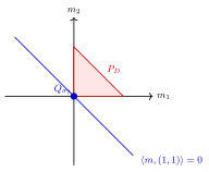
Example 21.13.82.A14927C0973A Let us consider the example example 21.13.15 again, we consider the subvariety corresponding to $\sigma _7$. We have
F8805F2A5BD021.13.83 The face $Q_{\sigma _7}=\{ m\in P_ D:\langle m,(1,1)\rangle =0\} $ is the single point $\{ (0,0)\} $, of dimension $0$ rather than the expected $1$.
We find that $\dim Q_{\sigma _7}=0$, but the expected dimension is $2-1=1$. So the corresponding divisor, namely the exceptional divisor on $\mathrm{Bl}_0\mathbb {P}^2$ is in the non-Kähler locus. Similarly, we can verify that the non-Kähler locus consists only of this divisor.
Finally, we compute the mixed volumes of Newton bodies.
Theorem 21.13.84.38F3E4DFCD04 Take $T$-invariant big divisors $D_1,\ldots ,D_ n$ on $X$. Consider $T_ c$-invariant closed positive $(1,1)$-currents $T_ i$ in $c_1(\mathcal{O}_ X(D_ i))$ for $i=1,\ldots ,n$. Then
In fact, assuming this, by induction, for each tuple of non-negative integers $C_1,\ldots ,C_ n$, we have
\[ \Delta \left( \sum _{i=1}^ n C_ i T_ i \right)=\sum _{i=1}^ n C_ i \Delta (T_ i). \]
Comparing the volumes, we have
\[ \operatorname{vol}\Delta \left( \sum _{i=1}^ n C_ i T_ i \right)=\sum _{i_1,\ldots ,i_ n=1}^ n C_{i_1}\cdots C_{i_ n} \operatorname{vol}\left(\Delta \left(T_{i_1}\right),\ldots ,\Delta \left(T_{i_ n}\right)\right). \]
On the other hand, by proposition 21.13.28, the $\mathcal{I}$-goodness of toric singularities example 18.1.56, and proposition 18.1.27, we have
\[ n! \operatorname{vol}\Delta \left( \sum _{i=1}^ n C_ i T_ i \right)=\operatorname{vol}\left( \sum _{i=1}^ n C_ i T_ i \right)=\sum _{i_1,\ldots ,i_ n=1}^ n C_{i_1}\cdots C_{i_ n} \operatorname{vol}\left(T_{i_1},\ldots ,T_{i_ n}\right). \]
Comparing the coefficients of the above two expressions, we conclude (21.13.85).
It only remains to establish (21.13.86). For this purpose, we fix smooth $T_ c$-invariant Hermitian metrics $h_1$ and $h_2$ on $\mathcal{O}_ X(D_1)$ and $\mathcal{O}_ X(D_2)$ respectively. Correspondingly, take $h_1\otimes h_2$ as the reference Hermitian metric on $\mathcal{O}_ X(D_1+D_2)$. Write
We choose the rational section of $\mathcal O_ X(D_1+D_2)$ to be $s_{D_1}\otimes s_{D_2}$. With this choice and with the reference metric $h_1\otimes h_2$, the normalization (21.13.23) gives
Take $\varphi _ i\in \mathrm{PSH}_{\mathrm{tor}}(X,\theta _ i)$ with $T_ i=\theta _ i+\mathrm{dd}^{\mathrm{c}}\varphi _ i$ for $i=1,2$. Then $F_{\varphi _1}+F_{\varphi _2}$ is a candidate for $F_{\varphi _1+\varphi _2}$; see (21.13.26). Therefore, (21.13.86) follows from the equality of closed gradient images proved in 21.11.47.
$\square$
Cite this page
Comments
Corrections, questions, and mathematical discussion are welcome. Sign in with GitHub to comment. Comments are public.
 Pome
Pome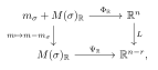
Comments
Corrections, questions, and mathematical discussion are welcome. Sign in with GitHub to comment. Comments are public.