Pome

22.1 Non-Archimedean pluripotential theory1E9C5D0261FD

1E9C5D0261FD

This chapter develops a non-Archimedean pluripotential theory for compact Kähler manifolds. In the projective setting, Boucksom and Jonsson constructed a space of non-Archimedean psh metrics on the Berkovich analytification of a polarized variety. Our approach starts instead from the analytic objects developed in the previous chapters: $\mathcal I$-model test curves and their operations. The resulting theory agrees with the Boucksom–Jonsson theory in the projective case.

The guiding idea is the Ross–Witt Nyström correspondence. A geodesic ray can be encoded by a test curve, and the $\mathcal I$-model version of this construction retains precisely the multiplier-ideal information relevant to algebraic approximation. For a pseudo-effective class $\{ \theta \} $, we define a non-Archimedean potential as an inverse system of $\mathcal I$-model test curves in the big classes $\{ \theta +\omega \} $, where $\omega $ ranges over Kähler forms. The transition maps are given by the $\mathcal I$-envelope.

After the definition, we develop the basic operations on non-Archimedean potentials. Sums, translations, maxima, suprema, infima and rescalings are induced from the corresponding operations on test curves. We also define the non-Archimedean volume and prove its basic monotonicity and continuity properties.

The next part of the chapter constructs the Duistermaat–Heckman measure of a non-Archimedean potential based on the theory of Okounkov bodies developed in section 19.1. It is defined through Okounkov test curves and is shown to be independent of the chosen flag.

The final part compares this construction with the Boucksom–Jonsson theory. In the projective case, we define the analytification of our non-Archimedean potentials and prove that the resulting space is naturally identified with the Boucksom–Jonsson space of psh non-Archimedean metrics.

The present chapter is logically based on the test-curve formalism of section 17.11, especially the $\mathcal I$-model theory of section 17.14 and the operations of section 17.15. It is largely independent of section 21.13, section 18.28, while the comparison with Boucksom–Jonsson uses the non-Archimedean theory recalled in subsection 22.1.64.

22.1.1 The definition of non-Archimedean metricsFB3B4C37DD45

Let $X$ be a connected compact Kähler manifold of dimension $n$. Let $\textup{Käh}(X)$ be the set of Kähler forms on $X$ with the partial order given as follows: We say $\omega \preceq \omega '$ if $\omega \geq \omega '$. Note that the partially ordered set $\textup{Käh}(X)$ is a directed set.

Let $\theta $ be a closed smooth real $(1,1)$-form representing a pseudo-effective cohomology class.

Definition 22.1.2.657951EB240B We define

\[ \mathrm{PSH}^{\mathrm{NA}}(X,\theta )=\varprojlim _{\omega \in \textup{Käh}(X)} \mathrm{PSH}^{\mathrm{NA}}(X,\theta +\omega )_{>0}{}^{\href{#sgpt-a0000106603}{1}} \]

in the category of sets, where the transition maps are given as follows: Suppose that $\omega ,\omega '\in \textup{Käh}$ and $\omega \geq \omega '$. Then the transition map is defined in proposition 17.14.6:

A99876729E5F 22.1.3
\begin{equation} P_{\theta +\omega }[\bullet ]_{\mathcal{I}}\colon \mathrm{PSH}^{\mathrm{NA}}(X,\theta +\omega ')_{>0}\rightarrow \mathrm{PSH}^{\mathrm{NA}}(X,\theta +\omega )_{>0}. \end{equation}

Note that the transition maps are compatible:

\[ P_{\theta +\omega ''}[P_{\theta +\omega '}[\varphi ]_\mathcal {I}]_\mathcal {I}=P_{\theta +\omega ''}[\varphi ]_\mathcal {I},\quad \forall \, \varphi \in \mathrm{PSH}^{\mathrm{NA}}(X,\theta +\omega )_{>0} \]

for $\omega \leq \omega '\leq \omega ''$, since both sides are $\mathcal{I}$-model and are $\mathcal{I}$-equivalent to $\varphi $.

Recall that $\mathrm{PSH}^{\mathrm{NA}}(X,\theta )_{>0}$ is defined in definition 17.14.1.

In general, when we denote an element in $\mathrm{PSH}^{\mathrm{NA}}(X,\theta )$ by $\Gamma $, its component in $\mathrm{PSH}^{\mathrm{NA}}(X,\theta +\omega )_{>0}$ ($\omega \in \textup{Käh}(X)$) will be written either as $\Gamma ^{\theta +\omega }$ or as $P_{\theta +\omega }[\Gamma ]_{\mathcal{I}}$.

Note that $\Gamma ^{\theta +\omega }_{\max }$ is independent of the choice of $\omega \in \textup{Käh}(X)$. We denote this common value by $\Gamma _{\max }$.

Remark 22.1.4.C864B821AD8B Thanks to proposition 17.14.3, for any other $\theta '$ representing $\{ \theta \} $, we have a canonical bijection

\[ \mathrm{PSH}^{\mathrm{NA}}(X,\theta )\xrightarrow {\sim }\mathrm{PSH}^{\mathrm{NA}}(X,\theta '). \]

Moreover, these bijections satisfy the cocycle condition. If we view the set of closed real smooth $(1,1)$-forms representing $\{ \theta \} $ as a category with a unique morphism between any two objects, then we can define

\[ \mathrm{PSH}^{\mathrm{NA}}(X,\{ \theta \} )=\varprojlim _{\theta } \mathrm{PSH}^{\mathrm{NA}}(X,\theta ). \]

This definition is independent of the choice of the explicit representative of the cohomology class $\{ \theta \} $.

However, given the fact that our notation is already quite heavy, we stick to the set $\mathrm{PSH}^{\mathrm{NA}}(X,\theta )$. The constructions below are independent of the choice of $\theta $ within its cohomology class.

Proposition 22.1.5.B80F3474DB2F Let $\Gamma \in \mathrm{PSH}^{\mathrm{NA}}(X,\theta )$. Then given $\omega ,\omega '\in \textup{Käh}(X)$ with $\omega \geq \omega '$, we have

\[ P_{\theta +\omega }\left[ \Gamma ^{\theta +\omega '}_{-\infty } \right]=P_{\theta +\omega }\left[ \Gamma ^{\theta +\omega '}_{-\infty } \right]_{\mathcal{I}} = \Gamma ^{\theta +\omega }_{-\infty }. \]

Proof. Since for any $\tau <\Gamma _{\max }$, the potential $\Gamma ^{\theta +\omega '}_{\tau }$ is $\mathcal{I}$-good by example 18.1.11, it follows that

\[ P_{\theta +\omega }\left[ \Gamma ^{\theta +\omega '}_{\tau } \right]=P_{\theta +\omega }\left[ \Gamma ^{\theta +\omega '}_{\tau } \right]_{\mathcal{I}}=\Gamma ^{\theta +\omega }_{\tau } \]

for all $\tau <\Gamma _{\max }$. Our assertion follows from proposition 16.4.9 and proposition 16.6.30. $\square$

Proposition 22.1.6.2CB4FA8703B1 There is a natural injective map

\[ \mathrm{PSH}^{\mathrm{NA}}(X,\theta )_{>0}\hookrightarrow \mathrm{PSH}^{\mathrm{NA}}(X,\theta ),\quad \Gamma \mapsto \left(P_{\theta +\omega }[\Gamma ]_{\mathcal{I}}\right)_{\omega \in \textup{Käh}(X)}. \]
In the sequel, we do not distinguish an element of $\mathrm{PSH}^{\mathrm{NA}}(X,\theta )_{>0}$ from its image in $\mathrm{PSH}^{\mathrm{NA}}(X,\theta )$. Note that given $\Gamma \in \mathrm{PSH}^{\mathrm{NA}}(X,\theta )_{>0}$, the value of $\Gamma _{\max }$ does not depend on whether we view it as an element of $\mathrm{PSH}^{\mathrm{NA}}(X,\theta )_{>0}$ or of $\mathrm{PSH}^{\mathrm{NA}}(X,\theta )$.

Proof. The map is well-defined by the compatibility of the transition maps. It suffices to argue its injectivity. Suppose that $\Gamma ,\Gamma '\in \mathrm{PSH}^{\mathrm{NA}}(X,\theta )_{>0}$ and

\[ P_{\theta +\omega }[\Gamma ]_{\mathcal{I}}=P_{\theta +\omega }[\Gamma ']_{\mathcal{I}} \]

for some Kähler form $\omega $ on $X$. Then $\Gamma _{\max }=\Gamma '_{\max }$ and for any $\tau <\Gamma _{\max }$, we have

\[ \Gamma _{\tau }\sim _{\mathcal{I}}\Gamma '_{\tau } \]

by proposition 16.8.17. It follows again from proposition 16.8.17 that

\[ \Gamma _{\tau }=\Gamma '_{\tau }. \]

This completes the proof. $\square$

Definition 22.1.7.A92D6DFAC0CF Let $\Gamma \in \mathrm{PSH}^{\mathrm{NA}}(X,\theta )$. We define its volume as follows:

\[ \operatorname{vol}\Gamma \coloneqq \lim _{\omega \in \textup{Käh}(X)} \int _ X \left(\theta +\omega +\mathrm{dd}^{\mathrm{c}}\Gamma ^{\theta +\omega }_{-\infty }\right)^ n\in [0,\infty ). \]
Observe that the net is decreasing, so the limit exists.

Proposition 22.1.8.47A4DA9EBA71 Let $\Gamma \in \mathrm{PSH}^{\mathrm{NA}}(X,\theta )_{>0}$. Then

\[ \operatorname{vol}\Gamma =\int _ X \left(\theta +\mathrm{dd}^{\mathrm{c}}\Gamma _{-\infty }\right)^ n. \]

Lemma 22.1.9.587EEDE88F4F Let $\Gamma \in \mathrm{PSH}^{\mathrm{NA}}(X,\theta )$, let $\omega $ be a Kähler form on $X$, and let $0<t\leq 1$. Then for every $\tau <\Gamma _{\max }$, we have

\[ \begin{aligned} & \int _ X \left(\theta +t\omega +\mathrm{dd}^{\mathrm{c}}\Gamma ^{\theta +t\omega }_{-\infty }\right)^ n-\int _ X \left(\theta +t\omega +\mathrm{dd}^{\mathrm{c}}\Gamma ^{\theta +t\omega }_{\tau }\right)^ n\\ \leq {}& \int _ X \left(\theta +\omega +\mathrm{dd}^{\mathrm{c}}\Gamma ^{\theta +\omega }_{-\infty }\right)^ n-\int _ X \left(\theta +\omega +\mathrm{dd}^{\mathrm{c}}\Gamma ^{\theta +\omega }_{\tau }\right)^ n. \end{aligned} \]

Proof. For $\sigma \in \{ -\infty ,\tau \} $, put

\[ S_ t^\sigma =\theta +t\omega +\mathrm{dd}^{\mathrm{c}}\Gamma ^{\theta +t\omega }_{\sigma }. \]

By the transition compatibility and proposition 22.1.5, example 18.1.11, proposition 16.3.10, projecting $\Gamma ^{\theta +t\omega }_{\sigma }$ to the class $\theta +\omega $ does not change the total mass computed in the larger class. Thus

\[ \int _ X \left(\theta +\omega +\mathrm{dd}^{\mathrm{c}}\Gamma ^{\theta +\omega }_{\sigma }\right)^ n = \int _ X \left(S_ t^\sigma +(1-t)\omega \right)^ n. \]

Expanding the right-hand side and subtracting the two identities for $\sigma =-\infty $ and $\sigma =\tau $, we get

\[ \begin{aligned} & \int _ X \left(\theta +\omega +\mathrm{dd}^{\mathrm{c}}\Gamma ^{\theta +\omega }_{-\infty }\right)^ n-\int _ X \left(\theta +\omega +\mathrm{dd}^{\mathrm{c}}\Gamma ^{\theta +\omega }_{\tau }\right)^ n\\ ={}& \sum _{a=0}^ n \binom {n}{a}(1-t)^{n-a} \left(\int _ X (S_ t^{-\infty })^ a\wedge \omega ^{n-a}-\int _ X (S_ t^\tau )^ a\wedge \omega ^{n-a}\right). \end{aligned} \]

Since $\Gamma ^{\theta +t\omega }_{-\infty }\geq \Gamma ^{\theta +t\omega }_{\tau }$, each summand is non-negative by the monotonicity theorem for mixed non-pluripolar products. Keeping only the term $a=n$ gives the desired inequality. $\square$

Lemma 22.1.10.9A2678C2C223 The image of the canonical injection

\[ \mathrm{PSH}^{\mathrm{NA}}(X,\theta )_{>0}\hookrightarrow \mathrm{PSH}^{\mathrm{NA}}(X,\theta ) \]

is given by the set of $\Gamma \in \mathrm{PSH}^{\mathrm{NA}}(X,\theta )$ with positive volume.

Proof. By proposition 22.1.8, every element in the image has positive volume.

Conversely, take $\Gamma \in \mathrm{PSH}^{\mathrm{NA}}(X,\theta )$ with positive volume. We want to construct $\Gamma '\in \mathrm{PSH}^{\mathrm{NA}}(X,\theta )_{>0}$ representing $\Gamma $.

Fix a Kähler form $\omega $ on $X$. Define

717C364BF812 22.1.11
\begin{equation} \Gamma '_{\tau }\coloneqq \lim _{k\to \infty }\Gamma ^{\theta +k^{-1}\omega }_{\tau },\quad \tau <\Gamma _{\max }. \end{equation}

We claim that it suffices to show

80067294986D 22.1.12
\begin{equation} \varliminf _{k\to \infty }\int _ X \left(\theta +k^{-1}\omega +\mathrm{dd}^{\mathrm{c}}\Gamma ^{\theta +k^{-1}\omega }_{\tau }\right)^ n>0 \end{equation}

for some $\tau <\Gamma _{\max }$. If this holds, then the argument of 17.12.6 implies that the same holds for all $\tau <\Gamma _{\max }$. Then proposition 16.4.4, proposition 16.6.29 guarantee that $\Gamma '\in \mathrm{PSH}^{\mathrm{NA}}(X,\theta )_{>0}$ and represents $\Gamma $.

It remains to argue (22.1.12). Let $\epsilon =\operatorname{vol}\Gamma >0$. Take $\tau <\Gamma _{\max }$ so that

\[ \int _ X \left(\theta +\omega +\mathrm{dd}^{\mathrm{c}}\Gamma ^{\theta +\omega }_{-\infty }\right)^ n-\int _ X \left(\theta +\omega +\mathrm{dd}^{\mathrm{c}}\Gamma ^{\theta +\omega }_{\tau }\right)^ n<\epsilon /2. \]

Therefore, by 22.1.9, for any $k\geq 1$,

\[ \int _ X \left(\theta +k^{-1}\omega +\mathrm{dd}^{\mathrm{c}}\Gamma ^{\theta +k^{-1}\omega }_{-\infty }\right)^ n-\int _ X \left(\theta +k^{-1}\omega +\mathrm{dd}^{\mathrm{c}}\Gamma ^{\theta +k^{-1}\omega }_{\tau }\right)^ n<\epsilon /2. \]

By the definition of $\operatorname{vol}\Gamma $, the first integral in the preceding line tends to $\epsilon $ as $k\to \infty $. Hence

\[ \varliminf _{k\to \infty }\int _ X \left(\theta +k^{-1}\omega +\mathrm{dd}^{\mathrm{c}}\Gamma ^{\theta +k^{-1}\omega }_{\tau }\right)^ n\geq \epsilon /2>0, \]

which proves (22.1.12). $\square$

Example 22.1.13.796F447D96B6 Fix $\varphi \in \mathrm{PSH}(X,\theta )$. We can define an associated non-Archimedean metric

\[ \Gamma ^{\varphi }\in \mathrm{PSH}^{\mathrm{NA}}(X,\theta ) \]

as follows:

  1. FB0E6FB2D0F7

    $\Gamma ^{\varphi }_{\max }=0$;

  2. 7A4B948C1C94

    for any $\omega \in \textup{Käh}(X)$ and any $\tau <0$, we set

    \[ \Gamma ^{\varphi ,\theta +\omega }_{\tau }=P_{\theta +\omega }[\varphi ]_{\mathcal{I}}. \]

Such non-Archimedean metrics are called homogeneous non-Archimedean metrics.

Observe that

\[ \operatorname{vol}\Gamma ^{\varphi }=\operatorname{vol}\theta _{\varphi }. \]

See proposition 18.1.27 and the footnote there.

Definition 22.1.14.CCAAC9DA4E2F Let $\omega $ be a closed real smooth positive $(1,1)$-form on $X$. We define the map

\[ P_{\theta +\omega }[\bullet ]_{\mathcal{I}}\colon \mathrm{PSH}^{\mathrm{NA}}(X,\theta )\rightarrow \mathrm{PSH}^{\mathrm{NA}}(X,\theta +\omega ) \]

as follows: Given $\Gamma \in \mathrm{PSH}^{\mathrm{NA}}(X,\theta )$, we define $P_{\theta +\omega }[\Gamma ]_{\mathcal{I}}$ as the element such that for any $\omega '\in \textup{Käh}(X)$, we have

\[ P_{\theta +\omega }[\Gamma ]_{\mathcal{I}}^{\theta +\omega +\omega '}=\Gamma ^{\theta +\omega +\omega '}. \]
It is straightforward to check that under the identification of proposition 22.1.6, the map $P_{\theta +\omega }[\bullet ]_{\mathcal{I}}$ extends the map (22.1.3).

Proposition 22.1.15.3943AA7119C5 The maps $P_{\theta +\omega }[\bullet ]_{\mathcal{I}}$ in definition 22.1.14 together induce a bijection

29D3530031C6 22.1.16
\begin{equation} \mathrm{PSH}^{\mathrm{NA}}(X,\theta )\xrightarrow {\sim } \varprojlim _{\omega \in \textup{Käh}(X)}\mathrm{PSH}^{\mathrm{NA}}(X,\theta +\omega ). \end{equation}

Proof. It is a tautology that the maps $P_{\theta +\omega }[\bullet ]_{\mathcal{I}}$ in definition 22.1.14 are compatible with the transition maps. So the map (22.1.16) is well-defined. It is injective by the same argument as proposition 22.1.6. We argue the surjectivity.

By unfolding the definitions, an object in the target of (22.1.16) is an assignment: With each $\omega \in \textup{Käh}(X)$, we associate a family $(\Gamma ^{\omega ,\omega '})_{\omega '\in \textup{Käh}(X)}$ satisfying:

  1. 5067A37E976E

    $\Gamma ^{\omega ,\omega '}\in \mathrm{PSH}^{\mathrm{NA}}(X,\theta +\omega +\omega ')_{>0}$ for each $\omega ,\omega '\in \textup{Käh}(X)$;

  2. CDB9ED278B54

    for each $\omega ,\omega ',\omega ''\in \textup{Käh}(X)$ satisfying $\omega ''\geq \omega '$, we have

    \[ P_{\theta +\omega +\omega ''}\left[\Gamma ^{\omega ,\omega '}\right]_{\mathcal{I}}=\Gamma ^{\omega ,\omega ''}; \]
  3. 3EBB3E3A9CF6

    for each $\omega ,\omega ',\omega ''\in \textup{Käh}(X)$ satisfying $\omega \leq \omega '$, we have

    \[ P_{\theta +\omega '+\omega ''}\left[\Gamma ^{\omega ,\omega ''}\right]_{\mathcal{I}}=\Gamma ^{\omega ',\omega ''}. \]

The preimage of such an object is given by the family $(\Gamma ^{\theta +\omega })_{\omega \in \textup{Käh}(X)}$ given by

\[ \Gamma ^{\theta +\omega }=\Gamma ^{\omega /2,\omega /2}. \]

The fact that the image of $\Gamma $ is as expected follows directly from the definitions. $\square$

With an almost identical argument involving proposition 16.4.4, we get

Proposition 22.1.17.817C1BB3E570 The maps $P_{\theta +\omega }[\bullet ]_{\mathcal{I}}$ in definition 22.1.14 and the injective maps proposition 22.1.6 together induce bijections

258B0F2A2F95 22.1.18
\begin{equation} \mathrm{PSH}^{\mathrm{NA}}(X,\theta )\xrightarrow {\sim } \varprojlim _{\omega }\mathrm{PSH}^{\mathrm{NA}}(X,\theta +\omega )_{>0}\xrightarrow {\sim } \varprojlim _{\omega }\mathrm{PSH}^{\mathrm{NA}}(X,\theta +\omega ), \end{equation}

where $\omega $ runs over either the partially ordered set of all smooth closed real positive $(1,1)$-forms with positive volume2 on $X$ or $\textup{Käh}(X)$.

Corollary 22.1.19.347399E47277 Let $\pi \colon Y\rightarrow X$ be a proper bimeromorphic morphism from a compact Kähler manifold $Y$. Then $\pi ^*$ induces a bijection

\[ \mathrm{PSH}^{\mathrm{NA}}(X,\theta )\xrightarrow {\sim } \mathrm{PSH}^{\mathrm{NA}}(Y,\pi ^*\theta ). \]

Proof. This follows immediately from proposition 22.1.17. $\square$

It is immediate to verify that $\pi ^*$ in corollary 22.1.19 extends the map proposition 17.14.4.

22.1.20 Operations on non-Archimedean metricsC20FEECB51B7

Let $X$ be a connected compact Kähler manifold of dimension $n$ and $\theta ,\theta ',\theta ''$ be closed real smooth $(1,1)$-forms on $X$ representing big cohomology classes.

This section relies heavily on section 17.15. We shall use the notions introduced in that section without further explanations.

Definition 22.1.21.DA2917901B54 Let $\Gamma \in \mathrm{PSH}^{\mathrm{NA}}(X,\theta )$, $\Gamma '\in \mathrm{PSH}^{\mathrm{NA}}(X,\theta ')$. We say $\Gamma \leq \Gamma '$ if for some $\omega \in \textup{Käh}(X)$, we have

\[ \Gamma ^{\theta +\omega } \leq \Gamma '{}^{\theta '+\omega }. \]
This notion is independent of the choice of $\omega $ thanks to 17.15.3. Moreover, we have the following:

Proposition 22.1.22.8C5A487B9CCC Let $\Gamma ,\Gamma '\in \mathrm{PSH}^{\mathrm{NA}}(X,\theta )$ and $\omega $ be a closed smooth positive $(1,1)$-form on $X$. Then the following are equivalent:

  1. A1B3616B9907

    $\Gamma \leq \Gamma '$;

  2. 3EAAE9BE6F17

    $P_{\theta +\omega }[\Gamma ]_{\mathcal{I}}\leq P_{\theta +\omega }[\Gamma ']_{\mathcal{I}}$.

Proof. This follows immediately from 17.15.3. $\square$

Observe that this definition coincides with the corresponding definition in definition 17.15.1 when $\Gamma ,\Gamma '\in \mathrm{PSH}^{\mathrm{NA}}(X,\theta )_{>0}$.

Proposition 22.1.23.F7D709A21AE1 Let $\Gamma ,\Gamma '\in \mathrm{PSH}^{\mathrm{NA}}(X,\theta )$. Assume that $\Gamma \leq \Gamma '$. Then

\[ \operatorname{vol}\Gamma \leq \operatorname{vol}\Gamma '. \]

Proof. It suffices to show that for any Kähler form $\omega $ on $X$, we have

\[ \operatorname{vol}\Gamma ^{\theta +\omega }_{-\infty }\leq \operatorname{vol}\Gamma '{}^{\theta +\omega }_{-\infty }, \]

which is an immediate consequence of theorem 13.13.11. $\square$

Definition 22.1.24.93939D1E527C Let $\Gamma \in \mathrm{PSH}^{\mathrm{NA}}(X,\theta )$ and $\Gamma '\in \mathrm{PSH}^{\mathrm{NA}}(X,\theta ')$. Then we define $\Gamma +\Gamma '\in \mathrm{PSH}^{\mathrm{NA}}(X,\theta +\theta ')$ as the unique element such that for any $\omega \in \textup{Käh}(X)$, we have

\[ \left( \Gamma +\Gamma ' \right)^{\theta +\theta '+2\omega }=\Gamma ^{\theta +\omega }+\Gamma '^{\theta '+\omega }. \]
This definition yields an element in $\mathrm{PSH}^{\mathrm{NA}}(X,\theta +\theta ')$ by 17.15.9 and it extends the definition in definition 17.15.4 by 17.15.9 as well.

Proposition 22.1.25.06DFF1DE1519 Let $\Gamma \in \mathrm{PSH}^{\mathrm{NA}}(X,\theta )$ and $\Gamma '\in \mathrm{PSH}^{\mathrm{NA}}(X,\theta ')$. Suppose that $\omega ,\omega '$ are two smooth closed positive $(1,1)$-forms on $X$. Then

\[ P_{\theta +\omega +\theta '+\omega '}[\Gamma +\Gamma ']_{\mathcal{I}}=P_{\theta +\omega }[\Gamma ]_{\mathcal{I}}+P_{\theta '+\omega '}[\Gamma ']_{\mathcal{I}}. \]

Proof. This is a direct consequence of 17.15.9. $\square$

Proposition 22.1.26.E9E94041F68D The operation $+$ is commutative and associative: For any $\Gamma \in \mathrm{PSH}^{\mathrm{NA}}(X,\theta )$, $\Gamma '\in \mathrm{PSH}^{\mathrm{NA}}(X,\theta ')$ and $\Gamma ''\in \mathrm{PSH}^{\mathrm{NA}}(X,\theta '')$, we have

\[ \Gamma +\Gamma '=\Gamma '+\Gamma ,\quad (\Gamma +\Gamma ')+\Gamma ''=\Gamma +(\Gamma '+\Gamma ''). \]

Proof. This is a direct consequence of proposition 17.15.7. $\square$

Definition 22.1.27.D1E32864F8F0 Let $\Gamma \in \mathrm{PSH}^{\mathrm{NA}}(X,\theta )$ and $C\in \mathbb {R}$. We define $\Gamma +C\in \mathrm{PSH}^{\mathrm{NA}}(X,\theta )$ as the unique element such that for any $\omega \in \textup{Käh}(X)$, we have

\[ \left( \Gamma +C \right)^{\theta +\omega }=\Gamma ^{\theta +\omega }+C. \]
It is obvious from definition 17.15.10 that $\Gamma +C\in \mathrm{PSH}^{\mathrm{NA}}(X,\theta )$. It is also obvious that this definition extends definition 17.15.10.

Proposition 22.1.28.ECFDC5EDD4F2 Let $\Gamma \in \mathrm{PSH}^{\mathrm{NA}}(X,\theta )$ and $C\in \mathbb {R}$. Suppose that $\omega $ is a smooth closed positive $(1,1)$-form on $X$. Then

\[ P_{\theta +\omega }[\Gamma ]_{\mathcal{I}}+C=P_{\theta +\omega }[\Gamma +C]_{\mathcal{I}}. \]

Proof. This is clear by definition. $\square$

Proposition 22.1.29.87CB041BFCA3 Let $\Gamma \in \mathrm{PSH}^{\mathrm{NA}}(X,\theta )$, $\Gamma '\in \mathrm{PSH}^{\mathrm{NA}}(X,\theta ')$ and $C,C'\in \mathbb {R}$. Then

  1. 80F4957A059F

    $(\Gamma +\Gamma ')+C=\Gamma +(\Gamma '+C)=(\Gamma +C)+\Gamma '$;

  2. 036FE960D3D0

    $\Gamma +(C+C')=(\Gamma +C)+C'$.

Proof. This is a direct consequence of proposition 17.15.11. $\square$

Proposition 22.1.30.11099644479B Let $\Gamma \in \mathrm{PSH}^{\mathrm{NA}}(X,\theta )$ and $C\in \mathbb {R}$. Then

\[ \operatorname{vol}\Gamma =\operatorname{vol}(\Gamma +C). \]

Proof. It suffices to show that for each Kähler form $\omega $ on $X$,

\[ \operatorname{vol}\Gamma ^{\theta +\omega }_{-\infty }=\operatorname{vol}(\Gamma +C)^{\theta +\omega }_{-\infty }, \]

which is obvious. $\square$

Definition 22.1.31.B819F1A85E09 Let $\Gamma ,\Gamma '\in \mathrm{PSH}^{\mathrm{NA}}(X,\theta )$, we define $\Gamma \lor \Gamma '\in \mathrm{PSH}^{\mathrm{NA}}(X,\theta )$ as the unique element such that for any $\omega \in \textup{Käh}(X)$, we have

\[ \left( \Gamma \lor \Gamma ' \right)^{\theta +\omega }=\Gamma ^{\theta +\omega }\lor \Gamma '^{\theta +\omega }. \]
It follows from 17.15.19 that $\Gamma \lor \Gamma '\in \mathrm{PSH}^{\mathrm{NA}}(X,\theta )$ and this definition extends the corresponding definition in definition 17.15.12.

Proposition 22.1.32.9CACCE9D7690 Let $\Gamma ,\Gamma '\in \mathrm{PSH}^{\mathrm{NA}}(X,\theta )$ and $\omega $ be a closed smooth positive $(1,1)$-form on $X$. Then

\[ P_{\theta +\omega }[\Gamma \lor \Gamma ']_{\mathcal{I}}=P_{\theta +\omega }[\Gamma ]_{\mathcal{I}}\lor P_{\theta +\omega }[\Gamma ']_{\mathcal{I}}. \]

Proof. This is a direct consequence of 17.15.19. $\square$

In particular, given a finite non-empty family $(\Gamma ^ i)_{i\in I}$ in $\mathrm{PSH}^{\mathrm{NA}}(X,\theta )$, we then define $\bigvee _{i\in I}\Gamma ^ i$ in the obvious way.

Proof. This is a direct consequence of corollary 17.15.17. $\square$

Definition 22.1.34.C172DAF1B3E6 Let $(\Gamma ^ i)_{i\in I}$ be a non-empty family in $\mathrm{PSH}^{\mathrm{NA}}(X,\theta )$. Assume that

AB5F1151338C 22.1.35
\begin{equation} \sup _{i\in I}\Gamma ^ i_{\max }<\infty . \end{equation}

Then we define $\operatorname *{sup}_{i\in I}{}\! {}^{*}\Gamma ^ i\in \mathrm{PSH}^{\mathrm{NA}}(X,\theta )$ as the unique element such that for any $\omega \in \textup{Käh}(X)$, we have

\[ \left( \operatorname *{sup}_{i\in I}{}\! {}^{*}\Gamma ^ i \right)^{\theta +\omega }=\operatorname *{sup}_{i\in I}{}\! {}^{*}\Gamma ^{i,\theta +\omega }. \]
It follows immediately from 17.15.30 that $\operatorname *{sup}_{i\in I}{}\! {}^{*}\Gamma ^ i\in \mathrm{PSH}^{\mathrm{NA}}(X,\theta )$ and this definition extends definition 17.15.25. Moreover, this definition clearly extends definition 22.1.31 as well.

Proposition 22.1.36.74CC0BF97B41 Let $(\Gamma ^ i)_{i\in I}$ be a non-empty family in $\mathrm{PSH}^{\mathrm{NA}}(X,\theta )$ satisfying (22.1.35). Assume that $\omega $ is a closed smooth positive $(1,1)$-form on $X$. Then

\[ P_{\theta +\omega }\left[ \operatorname *{sup}_{i\in I}{}\! {}^{*} \Gamma ^{i} \right]_{\mathcal{I}}= \operatorname *{sup}_{i\in I}{}\! {}^{*} P_{\theta +\omega }\left[ \Gamma ^{i} \right]_{\mathcal{I}}. \]

Proof. This is a direct consequence of 17.15.30. $\square$

We also have a non-Archimedean version of Choquet's lemma.

Proposition 22.1.37.21737B0303A5 Let $(\Gamma ^ i)_{i\in I}$ be a non-empty family in $\mathrm{PSH}^{\mathrm{NA}}(X,\theta )$ satisfying (22.1.35). Then there exists a countable subfamily $I'\subseteq I$ such that

\[ \operatorname *{sup}_{i\in I}{}\! {}^{*}\Gamma ^ i=\operatorname *{sup}_{i\in I'}{}\! {}^{*}\Gamma ^ i. \]

Proof. Fix a Kähler form $\omega _0$ on $X$. For each $m\geq 1$, proposition 17.15.31 gives a countable subfamily $I_ m\subseteq I$ such that

\[ \operatorname *{sup}_{i\in I}{}\! {}^{*}P_{\theta +m^{-1}\omega _0}[\Gamma ^ i]_{\mathcal{I}}=\operatorname *{sup}_{i\in I_ m}{}\! {}^{*}P_{\theta +m^{-1}\omega _0}[\Gamma ^ i]_{\mathcal{I}}. \]

Set $I'=\bigcup _{m\geq 1}I_ m$. This is countable. We claim that it works.

Let $\omega '\in \textup{Käh}(X)$. Choose $m$ so large that $\omega '\geq m^{-1}\omega _0$. By proposition 22.1.36 and the compatibility of the transition maps,

\[ \begin{aligned} \operatorname *{sup}_{i\in I}{}\! {}^{*}P_{\theta +\omega '}[\Gamma ^ i]_{\mathcal{I}} =& P_{\theta +\omega '}\left[\operatorname *{sup}_{i\in I}{}\! {}^{*}P_{\theta +m^{-1}\omega _0}[\Gamma ^ i]_{\mathcal{I}}\right]_{\mathcal{I}}\\ =& P_{\theta +\omega '}\left[\operatorname *{sup}_{i\in I'}{}\! {}^{*}P_{\theta +m^{-1}\omega _0}[\Gamma ^ i]_{\mathcal{I}}\right]_{\mathcal{I}}\\ =& \operatorname *{sup}_{i\in I'}{}\! {}^{*}P_{\theta +\omega '}[\Gamma ^ i]_{\mathcal{I}}. \end{aligned} \]

Thus the two non-Archimedean metrics have the same component in every class $\theta +\omega '$, and the assertion follows. $\square$

Proposition 22.1.38.938848E420F9 Let $(\Gamma ^ i)_{i\in I}$ be a non-empty family in $\mathrm{PSH}^{\mathrm{NA}}(X,\theta )$ satisfying (22.1.35). Let $C\in \mathbb {R}$. Then

\[ \operatorname *{sup}_{i\in I}{}\! {}^{*} (\Gamma ^ i+C)=\operatorname *{sup}_{i\in I}{}\! {}^{*} \Gamma ^ i+C. \]

Suppose that $(\Gamma '^ i)_{i\in I}$ is another family in $\mathrm{PSH}^{\mathrm{NA}}(X,\theta ')$ satisfying (22.1.35). Suppose that $\Gamma ^ i\leq \Gamma '^ i$ for all $i\in I$. Then

\[ \operatorname *{sup}_{i\in I}{}\! {}^{*}\Gamma ^ i\leq \operatorname *{sup}_{i\in I}{}\! {}^{*}\Gamma '^ i. \]

Proof. This is an immediate consequence of proposition 17.15.32. $\square$

Proposition 22.1.39.15E20104530B Let $(\Gamma ^ i)_{i\in I}$ be an increasing net in $\mathrm{PSH}^{\mathrm{NA}}(X,\theta )$ satisfying (22.1.35). Then

AA5696D80091 22.1.40
\begin{equation} \operatorname{vol}\left( \operatorname *{sup}_{i\in I}{}\! {}^{*} \Gamma ^ i \right)=\lim _{i\in I} \operatorname{vol}\Gamma ^ i. \end{equation}

Proof. The $\geq $ direction in (22.1.40) is a direct consequence of proposition 22.1.23. It remains to prove the reverse inequality.

Note that (22.1.40) holds when $\operatorname{vol}\Gamma ^ i>0$ for each $i\in I$, as a consequence of proposition 17.15.22, corollary 16.9.12 and theorem 16.9.57.

In particular, for each Kähler form $\omega $ on $X$, we have

\[ \operatorname{vol}\left( \operatorname *{sup}_{i\in I}{}\! {}^{*} \Gamma ^{i,\theta +\omega } \right)=\lim _{i\in I} \operatorname{vol}\Gamma ^{i,\theta +\omega }. \]

For our purpose, we need to show that for any $\epsilon >0$, we can find $\omega $ so that

\[ \sup _{i\in I} \operatorname{vol}\Gamma ^{i,\theta +\omega }<\sup _{i\in I} \operatorname{vol}\Gamma ^{i}+\epsilon . \]

We shall show that it is possible to choose $\omega $ so that the stronger statement holds:

\[ \operatorname{vol}\Gamma ^{i,\theta +\omega }<\operatorname{vol}\Gamma ^{i}+\epsilon ,\quad \forall i\in I. \]

Equivalently, we need to choose $\omega $ so that for any Kähler form $\omega '$ on $X$ dominated by $\omega $, we have

\[ \operatorname{vol}\Gamma ^{i,\theta +\omega }_{-\infty }<\operatorname{vol}\Gamma ^{i,\theta +\omega '}_{-\infty }+\epsilon /2,\quad \forall i\in I. \]

Fix a Kähler form $\omega _0$ on $X$ and a Kähler form $\Omega $ such that $\Omega \geq \theta +\omega _0$. It is enough to take $\omega =\delta \omega _0$ for some $\delta \in (0,1)$. If $\omega '$ is dominated by $\omega $, then $\theta +\omega '\leq \Omega $. Set

\[ T_ i\coloneqq \theta +\omega '+\mathrm{dd}^{\mathrm{c}}\Gamma ^{i,\theta +\omega '}_{-\infty }. \]

By the transition compatibility and proposition 17.12.19, the potential $\Gamma ^{i,\theta +\omega }_{-\infty }$ has the same $P$-singularity type in the class $\theta +\omega $ as $\Gamma ^{i,\theta +\omega '}_{-\infty }$. Hence its mass can be computed as

\[ \int _ X\left(\theta +\omega +\mathrm{dd}^{\mathrm{c}}\Gamma ^{i,\theta +\omega '}_{-\infty }\right)^ n=\int _ X \left(T_ i+\omega -\omega '\right)^ n. \]

Therefore,

\[ \begin{aligned} \operatorname{vol}\Gamma ^{i,\theta +\omega }_{-\infty }-\operatorname{vol}\Gamma ^{i,\theta +\omega '}_{-\infty } =& \int _ X \left(T_ i+\omega -\omega '\right)^ n-\int _ X T_ i^ n\\ =& \sum _{a=0}^{n-1} \binom {n}{a} \int _ X T_ i^ a\wedge \left( \omega -\omega '\right)^{n-a}\\ \leq & \sum _{a=0}^{n-1} \binom {n}{a} \int _ X \Omega ^ a\wedge \omega ^{n-a}. \end{aligned} \]

In the last inequality we used the facts that $0\leq \omega -\omega '\leq \omega $ and $\theta +\omega '\leq \Omega $, and the monotonicity theorem theorem 13.13.11. We can choose $\omega $ so that the right-hand side is less than $\epsilon /2$. Our assertion then follows. $\square$

Definition 22.1.41.65E2E07550F1 Let $(\Gamma ^ i)_{i\in I}$ be a decreasing net in $\mathrm{PSH}^{\mathrm{NA}}(X,\theta )$. Assume that

827FE14EA1A0 22.1.42
\begin{equation} \inf _{i\in I}\Gamma ^ i_{\max }>-\infty , \end{equation}

then we define $\inf _{i\in I}\Gamma ^ i\in \mathrm{PSH}^{\mathrm{NA}}(X,\theta )$ as the unique element such that for each $\omega \in \textup{Käh}(X)$, we have

341067287939 22.1.43
\begin{equation} \left( \inf _{i\in I}\Gamma ^ i \right)^{\theta +\omega }=\inf _{i\in I} \Gamma ^{i,\theta +\omega }. \end{equation}
We observe that
\[ \left( \inf _{i\in I}\Gamma ^ i \right)^{\theta +\omega }\in \mathrm{PSH}^{\mathrm{NA}}(X,\theta +\omega )_{>0}. \]

This follows from proposition 17.15.40. Moreover, by 17.15.41, we have $\inf _{i\in I}\Gamma ^ i\in \mathrm{PSH}^{\mathrm{NA}}(X,\theta )$, and this definition extends definition 17.15.37.

In general,

\[ \operatorname{vol}\left( \inf _{i\in I}\Gamma ^ i \right)\leq \lim _{i\in I} \operatorname{vol}\Gamma ^ i \]

as a consequence of proposition 22.1.23. But the reverse inequality fails in general.

Proposition 22.1.44.07B251D899EF Let $(\Gamma ^ i)_{i\in I}$ be a decreasing net in $\mathrm{PSH}^{\mathrm{NA}}(X,\theta )$ satisfying (22.1.42). Assume that $\omega $ is a closed smooth positive $(1,1)$-form on $X$. Then

\[ P_{\theta +\omega }\left[ \inf _{i\in I} \Gamma ^{i} \right]_{\mathcal{I}}= \inf _{i\in I} P_{\theta +\omega }\left[ \Gamma ^{i} \right]_{\mathcal{I}}. \]

Proof. This follows from 17.15.41. $\square$

Proposition 22.1.45.C8734FD15163 Let $(\Gamma ^ i)_{i\in I}$ be a decreasing net in $\mathrm{PSH}^{\mathrm{NA}}(X,\theta )$ satisfying (22.1.42). Let $C\in \mathbb {R}$. Then

\[ \inf _{i\in I} (\Gamma ^ i+C)=\inf _{i\in I} \Gamma ^ i+C. \]

Suppose that $(\Gamma '^ i)_{i\in I}$ is another decreasing net in $\mathrm{PSH}^{\mathrm{NA}}(X,\theta ')$ satisfying (22.1.42). Suppose that $\Gamma ^ i\leq \Gamma '^ i$ for all $i\in I$. Then

\[ \inf _{i\in I}\Gamma ^ i\leq \inf _{i\in I}\Gamma '^ i. \]

Proof. This is clear by definition. $\square$

Definition 22.1.46.EB1311598A32 Let $\Gamma \in \mathrm{PSH}^{\mathrm{NA}}(X,\theta )$ and $\lambda \in \mathbb {R}_{>0}$. Then we define $\lambda \Gamma \in \mathrm{PSH}^{\mathrm{NA}}(X,\lambda \theta )$ as the unique element such that for any $\omega \in \textup{Käh}(X)$, we have

\[ \left( \lambda \Gamma \right)^{\lambda \theta +\omega }=\lambda \Gamma ^{\theta +\lambda ^{-1}\omega }. \]
It follows immediately from 17.15.36 that $\lambda \Gamma \in \mathrm{PSH}^{\mathrm{NA}}(X,\lambda \theta )$ and this definition extends definition 17.15.33.

Proposition 22.1.47.68FB6124EEB2 Let $\Gamma \in \mathrm{PSH}^{\mathrm{NA}}(X,\theta )$ and $\lambda \in \mathbb {R}_{>0}$. Then for any closed smooth positive $(1,1)$-form $\omega $ on $X$, we have

\[ P_{\lambda \theta +\omega }[\lambda \Gamma ]_{\mathcal{I}}=\lambda P_{\theta +\lambda ^{-1}\omega }[\Gamma ]_{\mathcal{I}}. \]

Proof. This follows immediately from 17.15.36. $\square$

Proposition 22.1.48.EDFB2682E78E Let $\Gamma \in \mathrm{PSH}^{\mathrm{NA}}(X,\theta )$, $\Gamma '\in \mathrm{PSH}^{\mathrm{NA}}(X,\theta ')$, $C\in \mathbb {R}$ and $\lambda ,\lambda '>0$, we have

\[ \begin{aligned} \lambda (\Gamma +\Gamma ')=& \lambda \Gamma +\lambda \Gamma ',\\ (\lambda \lambda ')\Gamma =& \lambda (\lambda '\Gamma ),\\ \lambda (\Gamma +C)=& \lambda \Gamma +\lambda C. \end{aligned} \]

Suppose that $(\Gamma ^ i)_{i\in I}$ is a non-empty family in $\mathrm{PSH}^{\mathrm{NA}}(X,\theta )$ satisfying (22.1.35). Then

\[ \lambda \left( \operatorname *{sup}_{i\in I}{}\! {}^{*}\Gamma ^ i \right)=\operatorname *{sup}_{i\in I}{}\! {}^{*}(\lambda \Gamma ^ i). \]

If $(\Gamma ^ i)_{i\in I}$ is a decreasing net in $\mathrm{PSH}^{\mathrm{NA}}(X,\theta )$ satisfying (22.1.42), then

\[ \lambda \left( \inf _{i\in I}\Gamma ^ i \right)=\inf _{i\in I}(\lambda \Gamma ^ i). \]

Proof. Everything except the last assertion follows from proposition 17.15.35. The last assertion follows directly from the definition. $\square$

Proposition 22.1.49.1743F9AEA475 Let $\Gamma \in \mathrm{PSH}^{\mathrm{NA}}(X,\theta )$ and $\lambda \in \mathbb {R}_{>0}$. Then

\[ \operatorname{vol}\left( \lambda \Gamma \right)=\lambda ^ n \operatorname{vol}\Gamma . \]

Proof. This is clear by definition. $\square$

Definition 22.1.50.C0E37055D126 Let $\Gamma \in \mathrm{PSH}^{\mathrm{NA}}(X,\theta )$. Let $Y\subseteq X$ be an irreducible analytic subset. We say that the trace operator of $\Gamma $ along $Y$ is well-defined if

\[ \nu \left(\Gamma _{\tau }^{\theta +\omega },Y\right)=0 \]

for all sufficiently negative $\tau $ and every $\omega \in \textup{Käh}(X)$. We define

\[ \left(\operatorname{Tr}_ Y(\Gamma )\right)_{\max }\coloneqq \sup \left\{ \tau <\Gamma _{\max }: \nu \left(\Gamma _{\tau }^{\theta +\omega },Y\right)=0\right\} . \]

Here $\omega $ is any Kähler form on $X$; this number is independent of the choice of $\omega $ by the compatibility of the transition maps.

In this case, we define $\operatorname{Tr}_ Y(\Gamma )\in \mathrm{PSH}^{\mathrm{NA}}(\widetilde{Y},\theta |_{\widetilde{Y}})$3 as the unique element such that for any $\omega \in \textup{Käh}(\widetilde{Y})$, the component

6697E3349082 22.1.51
\begin{equation} \operatorname{Tr}_ Y(\Gamma )^{\theta |_{\widetilde{Y}}+\omega }\in \mathrm{PSH}^{\mathrm{NA}}(\widetilde{Y},\theta |_{\widetilde{Y}}+\omega )_{>0} \end{equation}

is defined as follows:

  1. 5517A8C43D97

    We let

    284D786E2B4E 22.1.52
    \begin{equation} \left( \operatorname{Tr}_ Y(\Gamma )^{\theta |_{\widetilde{Y}}+\omega } \right)_{\max }=\left(\operatorname{Tr}_ Y(\Gamma )\right)_{\max }; \end{equation}
  2. E0B260D169B4

    for each $\tau \in \mathbb {R}$ less than $\left(\operatorname{Tr}_ Y(\Gamma )\right)_{\max }$, we define

    \[ \operatorname{Tr}_ Y(\Gamma )^{\theta |_{\widetilde{Y}}+\omega }_{\tau }\coloneqq P_{\theta |_{\widetilde{Y}}+\omega }\left[ \operatorname{Tr}_ Y^{\theta +\tilde{\omega }}\left(\Gamma ^{\theta +\tilde{\omega }}_{\tau }\right) \right]_{\mathcal{I}}, \]

    where $\tilde{\omega }$ is an arbitrary Kähler form on $X$ such that $\omega \geq \tilde{\omega }|_{\widetilde{Y}}$.

It follows from [Proposition 3.6, GK20] that $\widetilde{Y}$ is a normal Kähler space and hence $\tilde{\omega }$ exists. We observe that the choice of the trace operator $\operatorname{Tr}_ Y^{\theta +\tilde{\omega }}\left(\Gamma ^{\theta +\tilde{\omega }}_{\tau }\right)$ is irrelevant since two different choices are $\mathcal{I}$-equivalent. Moreover, (22.1.51) holds as a consequence of proposition 20.2.8 and proposition 20.2.21. It is therefore clear that $\operatorname{Tr}_ Y(\Gamma )\in \mathrm{PSH}^{\mathrm{NA}}(\widetilde{Y},\theta |_{\widetilde{Y}})$. Here when $\widetilde{Y}$ is not smooth, we understand $\mathrm{PSH}^{\mathrm{NA}}(\widetilde{Y},\theta |_{\widetilde{Y}})$ as the set of non-Archimedean metrics on a resolution of $\widetilde{Y}$, which is independent of the choice of the resolution by proposition 20.2.21. See section 9.10 for more details.

Proposition 22.1.53.E7009D90BCC6 Let $\pi \colon Y\rightarrow X$ be a proper bimeromorphic morphism from a compact Kähler manifold $Y$. Then all definitions in this section are invariant under pullback to $Y$.

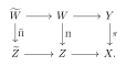
The meaning is clear in most cases. In the case of the trace operator, this means the following: Suppose that $Z\subseteq X$ is an analytic subset and $\Gamma \in \mathrm{PSH}^{\mathrm{NA}}(X,\theta )$ has non-trivial restriction to $Z$. Suppose that $Z$ is not contained in the non-isomorphism locus of $\pi $ so that the strict transform $W$ of $Z$ is defined. If we write $\Pi \colon W\rightarrow Z$ for the restriction of $\pi $ and $\widetilde{\Pi }\colon \widetilde{W}\rightarrow \widetilde{Z}$ the strict transform of $\Pi $, then we have
\[ \widetilde{\Pi }^* \operatorname{Tr}_ Z(\Gamma )=\operatorname{Tr}_ W(\pi ^*\Gamma ). \]

The relevant notations are summarized in the following diagram:
Mathematical diagram from the source

Proof. We only prove the assertion for the trace operator, as the other proofs are similar.

We shall use the notations above. Observe that for any closed positive smooth $(1,1)$-form $\omega $ on $X$ with positive mass, we have

\[ \left(\widetilde{\Pi }^* \operatorname{Tr}_ Z(\Gamma )\right)_{\max }=\left( \operatorname{Tr}_ Z(\Gamma )\right)_{\max }=\sup \left\{ \tau <\Gamma _{\max }: \nu \left(\Gamma ^{\theta +\omega }_{\tau },Z\right)=0 \right\} , \]

and

\[ \begin{aligned} \left(\operatorname{Tr}_ W(\pi ^*\Gamma )\right)_{\max }=& \sup \left\{ \tau <\Gamma _{\max }: \nu \left((\pi ^*\Gamma )^{\pi ^*\theta +\pi ^*\omega }_{\tau },W\right)=0 \right\} \\ =& \sup \left\{ \tau <\Gamma _{\max }: \nu \left(\pi ^*\Gamma ^{\theta +\omega }_{\tau },W\right)=0 \right\} \\ =& \sup \left\{ \tau <\Gamma _{\max }: \nu \left(\Gamma ^{\theta +\omega }_{\tau },Z\right)=0 \right\} . \end{aligned} \]

Here we implicitly used proposition 22.1.17. Therefore,

\[ \left(\widetilde{\Pi }^* \operatorname{Tr}_ Z(\Gamma )\right)_{\max }=\left(\operatorname{Tr}_ W(\pi ^*\Gamma )\right)_{\max }. \]

Let $\tau \in \mathbb {R}$ be less than this common value. Take a Kähler form $\omega _{\widetilde{Z}}$ (resp. $\omega _{\widetilde{W}}$) on $\widetilde{Z}$ (resp. $\widetilde{W}$). Take a Kähler form $\omega _ Y$ on $Y$ (resp. $\omega _ X$ on $X$) such that

\[ \omega _{\widetilde{Z}}\geq \omega _ X|_{\widetilde{Z}},\quad \omega _{\widetilde{W}} \geq \omega _ Y|_{\widetilde{W}},\quad \omega _ Y \geq \pi ^*\omega _ X. \]

We want to show that, after projection to the common background $(\pi ^*\theta )|_{\widetilde{W}}+\omega _{\widetilde{W}}$,

\[ P_{(\pi ^*\theta )|_{\widetilde{W}}+\omega _{\widetilde{W}}}\left[\widetilde{\Pi }^*\left(\operatorname{Tr}_ Z(\Gamma )^{\theta |_{\widetilde{Z}}+\omega _{\widetilde{Z}}}_\tau \right)\right]_{\mathcal I} \sim _ P \left(\operatorname{Tr}_ W(\pi ^*\Gamma )\right)^{(\pi ^*\theta )|_{\widetilde{W}}+\omega _{\widetilde{W}}}_\tau . \]

Unfolding the definitions, we reduce to

\[ \widetilde{\Pi }^* \operatorname{Tr}_ Z^{\theta +\omega _ X}\left( \Gamma ^{\theta +\omega _ X}_{\tau } \right)\sim _ P \operatorname{Tr}_{W}^{\pi ^*\theta +\omega _ Y}\left( \left( \pi ^*\Gamma \right)^{\pi ^*\theta +\omega _ Y}_{\tau }\right). \]

Using proposition 20.2.21, this is equivalent to

\[ \widetilde{\Pi }^* \operatorname{Tr}_ Z\left( \Gamma ^{\theta +\omega _ X}_{\tau } \right)\sim _ P \operatorname{Tr}_{W}\left( \left( \pi ^*\Gamma \right)^{\pi ^*\theta +\pi ^*\omega _ X}_{\tau }\right). \]

This is a consequence of 20.2.24. $\square$

22.1.54 Duistermaat–Heckman measures3C0D12E80020

Let $X$ be a connected compact Kähler manifold of dimension $n$ and $\theta $ be a closed real smooth $(1,1)$-form on $X$ representing a big cohomology class.

Definition 22.1.55.9ADEFD2FF381 Assume that $X$ admits a smooth flag $Y_{\bullet }$. Let $\Gamma \in \mathrm{PSH}^{\mathrm{NA}}(X,\theta )_{>0}$. The Duistermaat–Heckman measure $\operatorname{DH}(\Gamma )$ of $\Gamma $ is defined as

\[ \operatorname{DH}(\Gamma )\coloneqq n!\cdot \operatorname{DH}\left(\Delta _{Y_{\bullet }}(\theta ,\Gamma )\right). \]
Recall that $\Delta _{Y_{\bullet }}(\theta ,\Gamma )\in \mathrm{TC}(\Delta _{Y_{\bullet }}(\theta ,\Gamma _{-\infty }))$ is the Okounkov test curve defined in theorem 19.6.24. See definition 19.6.18 for the definition of the Duistermaat–Heckman measure of an Okounkov test curve.

Theorem 22.1.56.0AD7F80A793D Assume that $X$ admits a smooth flag $Y_{\bullet }$. The Duistermaat–Heckman measure $\operatorname{DH}(\Gamma )$ of $\Gamma \in \mathrm{PSH}^{\mathrm{NA}}(X,\theta )_{>0}$ in definition 22.1.55 is independent of the choice of the smooth flag $Y_{\bullet }$. Furthermore, for any $m\in \mathbb {Z}_{>0}$, the following moment identity holds:

A51020D58E6F 22.1.57
\begin{equation} \int _{\mathbb {R}}x^ m\operatorname{DH}(\Gamma )(x)=\Gamma _{\max }^ m\operatorname{vol}\Gamma +m\int _{-\infty }^{\Gamma _{\max }}\tau ^{m-1}\Bigl ( \operatorname{vol}(\theta +\mathrm{dd}^{\mathrm{c}}\Gamma _{\tau })-\operatorname{vol}\Gamma \Bigr )\, \mathrm{d}\tau , \end{equation}

and

51031202809C 22.1.58
\begin{equation} \int _{\mathbb {R}}\operatorname{DH}(\Gamma )=\operatorname{vol}\Gamma . \end{equation}
For each $m\in \mathbb {N}$, $\int _{\mathbb {R}}x^ m\operatorname{DH}(\Gamma )(x)$ is indeed $n!$ times the $m$-th moment of the random variable $G[\Delta _{Y_{\bullet }}(\theta ,\Gamma )]$, by definition 22.1.55, definition 19.6.18.

Proof. We observe that (22.1.57) holds by the computations in proposition 19.6.19 and theorem 19.5.26 1. It is independent of the choice of the flag. Furthermore, (22.1.58) follows immediately from theorem 19.5.26 1.

Assume first that $\Gamma $ is bounded. Since the Duistermaat–Heckman measure has bounded support in this case (cf. theorem 19.6.13), we conclude that $\operatorname{DH}(\Gamma )$ is uniquely determined.

By translating the parameter, it suffices to treat the case $\Gamma _{\max }=0$. Indeed, if $a=\Gamma _{\max }$ and

\[ \widetilde\Gamma _\tau \coloneqq \Gamma _{\tau +a}, \]

then $\widetilde\Gamma _{\max }=0$, and the associated test function is translated by $a$. Consequently,

\[ \operatorname{DH}(\Gamma )=(x\mapsto x+a)_*\operatorname{DH}(\widetilde\Gamma ). \]

Thus independence of the flag and the moment identity for $\widetilde\Gamma $ imply the corresponding assertions for $\Gamma $.

For each $\epsilon >0$, we define $\Gamma ^{\epsilon }\in \mathrm{PSH}^{\mathrm{NA}}(X,\theta )_{>0}$ as follows:

  1. 36B347B9186A

    Let $\Gamma ^{\epsilon }_{\max }=0$, and

  2. 12A1009F3470

    we set

    \[ \Gamma ^{\epsilon }_{\tau }= \begin{cases} \Gamma _{-\infty },& \text{ if }\tau \leq -\epsilon ^{-1},\\ P_{\theta }\left[ (1+\epsilon \tau )\Gamma _{\tau }-\epsilon \tau \Gamma _{-\infty } \right],& \text{ if }\tau \in \left(-\epsilon ^{-1},0\right). \end{cases} \]

Let us check that $\Gamma ^\epsilon $ is indeed an element of $\mathrm{PSH}^{\mathrm{NA}}(X,\theta )_{>0}$. The concavity and monotonicity in $\tau $ follow from proposition 16.4.2. Since the $\Gamma _\tau $'s are $\mathcal I$-model, they are $\mathcal I$-good by example 18.1.11; hence

\[ (1+\epsilon \tau )\Gamma _\tau -\epsilon \tau \Gamma _{-\infty } \]

is $\mathcal I$-good by proposition 18.1.17. Therefore its $P$-envelope is also its $\mathcal I$-envelope, and the corresponding level is $\mathcal I$-model. The value at $-\infty $ is $\Gamma _{-\infty }$. Thus $\Gamma ^\epsilon \in \mathrm{PSH}^{\mathrm{NA}}(X,\theta )_{>0}$.

For each fixed $\tau <0$, the argument of theorem 17.13.21 Step 3.3 gives

\[ \Gamma ^\epsilon _\tau \searrow \Gamma _\tau \quad \textup{as }\epsilon \to 0+. \]

By proposition 16.4.4 and corollary 16.9.14, this convergence is in $d_ S$. Hence theorem 19.5.26 4 gives

\[ \Delta _{Y_\bullet }(\theta ,\Gamma ^\epsilon _\tau )\xrightarrow {d_{\mathrm{Haus}}}\Delta _{Y_\bullet }(\theta ,\Gamma _\tau ) \]

for every $\tau <0$. Since

\[ \Gamma ^\epsilon _{-\infty }=\Gamma _{-\infty } \]

for all $\epsilon $, the underlying convex body is fixed. Therefore 19.6.22 applies and gives

\[ \operatorname{DH}(\Gamma ^\epsilon )\rightharpoonup \operatorname{DH}(\Gamma ). \]

It follows that $\operatorname{DH}(\Gamma )$ is independent of the choice of the flag. $\square$

More generally, when $X$ does not admit a smooth flag, we may choose a modification $\pi \colon Y\rightarrow X$ so that $Y$ admits a flag. We define

665B92171EA8 22.1.59
\begin{equation} \operatorname{DH}(\Gamma )\coloneqq \operatorname{DH}(\pi ^*\Gamma ). \end{equation}

It follows from theorem 19.5.26 5 that this measure is independent of the choice of $\pi $.

Proposition 22.1.60.492A145E9067 Let

\[ (\Gamma ^ i)_{i\geq 1}\subseteq \mathrm{PSH}^{\mathrm{NA}}(X,\theta )_{>0},\quad \Gamma \in \mathrm{PSH}^{\mathrm{NA}}(X,\theta )_{>0}. \]

Assume one of the following conditions holds:

  1. 577BE71DB8C5

    The sequence $(\Gamma ^ i)_{i\geq 1}$ is decreasing and $\Gamma =\inf _{i\geq 1}\Gamma ^ i$. Assume that

    E10A583B2E40 22.1.61
    \begin{equation} \operatorname{vol}\Gamma =\lim _{i\to \infty }\operatorname{vol}\Gamma ^ i. \end{equation}
  2. 75E1B24CB49A

    The sequence $(\Gamma ^ i)_{i\geq 1}$ is increasing and $\Gamma =\operatorname *{sup}_{i\geq 1}{}\! {}^{*}\Gamma ^ i$.

Then

636AFE1086C1 22.1.62
\begin{equation} \operatorname{DH}(\Gamma ^ i)\rightharpoonup \operatorname{DH}(\Gamma ). \end{equation}

Proof. We may assume that $X$ admits a smooth flag $Y_{\bullet }$.

Assume 1. Let

\[ \eta \coloneqq \inf _{i\geq 1}\Gamma ^ i_{-\infty }. \]

Since $\Gamma _\tau \leq \Gamma ^ i_{-\infty }$ for every $i$ and every $\tau <\Gamma _{\max }$, we have

\[ \Gamma _{-\infty }\leq \eta . \]

By proposition 16.4.4, the decreasing limit $\eta $ is model and

\[ \int _ X\theta _\eta ^ n=\lim _{i\to \infty }\int _ X\theta _{\Gamma ^ i_{-\infty }}^ n=\lim _{i\to \infty }\operatorname{vol}\Gamma ^ i. \]

Using (22.1.61), this equals

\[ \operatorname{vol}\Gamma =\int _ X\theta _{\Gamma _{-\infty }}^ n. \]

Since $\Gamma _{-\infty }\leq \eta $ and both potentials are model, proposition 16.8.7 gives

\[ \Gamma _{-\infty }=\eta . \]

Thus

\[ \Gamma _{-\infty }=\inf _{i\geq 1}\Gamma ^ i_{-\infty }. \]

We want to derive (22.1.62) from 19.6.22. It boils down to prove the following: For any $\tau <\Gamma _{\max }$, we have

\[ \Delta _{Y_{\bullet }}(\theta ,\Gamma ^ i_{\tau })\xrightarrow {d_{\mathrm{Haus}}} \Delta _{Y_{\bullet }}(\theta ,\Gamma _{\tau }). \]

For fixed $\tau <\Gamma _{\max }$, the potentials $\Gamma ^ i_\tau $ decrease to $\Gamma _\tau $. By proposition 16.4.4, their masses converge to the mass of $\Gamma _\tau $; hence $\Gamma ^ i_\tau \xrightarrow {d_ S}\Gamma _\tau $ by corollary 16.9.14. Applying the continuity of the partial Okounkov body map, theorem 19.5.26 4, gives

\[ \Delta _{Y_{\bullet }}(\theta ,\Gamma ^ i_{\tau })\xrightarrow {d_{\mathrm{Haus}}}\Delta _{Y_{\bullet }}(\theta ,\Gamma _{\tau }). \]

The proof under the assumption 2 is similar. We only need to apply 19.6.23 instead of 19.6.22. $\square$

Remark 22.1.63.CF750A31909E When $\{ \theta \} $ is a Hodge class and $\Gamma $ is induced by a test configuration as in example 17.14.10 and 17.14.14, our Duistermaat–Heckman measure coincides with the more traditional definition of [Section 3.2, BHJ17]. This is explained in [Remark 7.17, Xia21].

22.1.65 A brief recap of Boucksom–Jonsson's theory82D43892E8F6

Non-Archimedean plurisubharmonic metrics are defined by decreasing limits of Fubini–Study functions on the analytification of a projective variety. The results below relate these metrics to test curves.

22.1.66 Valuations618C84432CDA

Let $X$ be an irreducible reduced variety over $\mathbb {C}$ of dimension $n$. We recall the Berkovich analytification $X^{\mathrm{An}}$ of $X$ with respect to the trivial valuation on $\mathbb {C}$.

Definition 22.1.67.433FF564E9A3 A (real-valued) valuation on $X$ (or a valuation of $\mathbb {C}(X)$) is a map $v\colon \mathbb {C}(X)\rightarrow (-\infty ,\infty ]$ satisfying the following conditions:

  1. 8EDEF9CF138B

    For $f\in \mathbb {C}(X)$, $v(f)=\infty $ if and only if $f=0$;

  2. 3ACA653FD4D8

    For $f,g\in \mathbb {C}(X)$, $v(fg)=v(f)+v(g)$;

  3. 4C1AC87714F3

    For $f,g\in \mathbb {C}(X)$, $v(f+g)\geq v(f)\land v(g)$;

  4. C9D9521A044A

    For $c\in \mathbb {C}^{\times }$, $v(c)=0$.

The set of valuations on $X$ is denoted by $X^{\mathrm{val}}$. The center of a valuation $v$ is the scheme-theoretic point $c=c(v)$ of $X$ such that $v\geq 0$ on $\mathcal{O}_{X,c}$ and $v>0$ on the maximal ideal $\mathfrak {m}_{X,c}$ of $\mathcal{O}_{X,c}$. The center is unique if it exists, and it exists if $X$ is proper.

In the remainder of this section, we assume that $X$ is projective.

As a set, $X^{\mathrm{An}}$ is the set of semi-valuations on $X$, in other words, real-valued valuations $v$ on irreducible reduced subvarieties $Y$ of $X$ that are trivial on $\mathbb {C}$. We call $Y$ the support of the semi-valuation $v$. In other words,

\[ X^{\mathrm{An}}=\coprod _{Y} Y^{\mathrm{val}}. \]

We will write $v_{\mathrm{triv}}\in X^{\mathrm{An}}$ for the trivial valuation on $X$: $v_{\mathrm{triv}}(f)=0$ for any $f\in \mathbb {C}(X)^{\times }$.

We endow $X^{\mathrm{An}}$ with the coarsest topology such that

  1. 3E9AB9B11483

    for any Zariski open subset $U\subseteq X$, the subset $U^{\mathrm{An}}$ of $X^{\mathrm{An}}$ consisting of semi-valuations whose supports meet $U$ is open;

  2. 16DC97C2CD0A

    for each Zariski open subset $U\subseteq X$ and each $f\in \mathrm{H}^0(U,\mathcal{O}_ X)$ (here $\mathcal{O}_ X$ is the sheaf of regular functions), the map $|f|\colon U^{\mathrm{An}}\rightarrow \mathbb {R}$ sending $v$ to $\exp (-v(f))$ is continuous.

We will be most interested in divisorial valuations. Recall that a divisorial valuation on $X$ is a valuation of the form $t\operatorname{ord}_ E$, where $t\in \mathbb {Q}_{>0}$ and $E$ is a prime divisor over $X$. The set of divisorial valuations on $X$ is denoted by $X^{\operatorname{div}}$. When $\mathbb {Q}_{>0}$ is replaced by $\mathbb {R}_{>0}$, we can similarly define a space $X^{\operatorname{div}}_{\mathbb {R}}$.

Given any coherent ideal $\mathfrak {a}$ on $X$ and any $v\in X^{\mathrm{An}}$, we define

18B5288E3A41 22.1.68
\begin{equation} v(\mathfrak {a})\coloneqq \min \{ v(f):f\in \mathfrak {a}_{c(v)}\} \in [0,\infty ], \end{equation}

where $c(v)$ is the center of the valuation $v$ on $X$.

Given any valuation $v$ on $X$, the Gauss extension of $v$ is a valuation $\sigma (v)$ on $X\times \mathbb {A}^1$:

3B8E87503101 22.1.69
\begin{equation} \sigma (v)\left(\sum _ i f_ i t^ i\right)\coloneqq \min _ i (v(f_ i)+i). \end{equation}

Here $t$ is the standard coordinate on $\mathbb {A}^1=\operatorname{Spec}\mathbb {C}[t]$. The key property is that when $v$ is a divisorial valuation, then so is $\sigma (v)$. See [Lemma 4.2, BHJ17].

22.1.70 Non-Archimedean plurisubharmonic functions3CE1C3E79114

Let $X$ be an irreducible complex projective variety of dimension $n$ and $L$ be a holomorphic pseudo-effective $\mathbb {Q}$-line bundle on $X$. Through the GAGA morphism $X^{\mathrm{An}}\rightarrow X$ of ringed spaces, $L$ can be pulled back to an analytic line bundle $L^{\mathrm{An}}$ on $X$. The purpose of this section is to study the psh metrics on $L^{\mathrm{An}}$. This description avoids the direct treatment of $L^{\mathrm{An}}$ itself.

We define $\mathcal{H}^{\mathrm{gf}}_{\mathbb {Q}}(L^{\mathrm{An}})$, the set of (rational) generically finite Fubini–Study functions $\phi \colon X^{\mathrm{An}}\rightarrow [-\infty ,\infty )$ that are of the following form:

13.37
\begin{equation} \phi =\frac{1}{m}\max _ j \{ \log |s_ j|+\lambda _ j\} . \end{equation}

Here $m\in \mathbb {Z}_{>0}$ is an integer such that $L^ m$ is a line bundle, the $s_ j$'s are a finite collection of non-zero sections in $\mathrm{H}^0(X,L^ m)$, and $\lambda _ j\in \mathbb {Q}$. We follow the convention of Boucksom–Jonsson by writing $\log |s_ j|(v)=-v(s_ j)$.

Definition 22.1.71 .EEADED50AAC3 A plurisubharmonic metric (or psh metric for short) on $L^{\mathrm{An}}$ is a function $\phi \colon X^{\mathrm{An}}\rightarrow [-\infty ,\infty )$ that is not identically $-\infty $, and is the pointwise limit of a decreasing net $(\phi _ i)_{i\in I}$, where $\phi _ i\in \mathcal{H}^{\mathrm{gf}}_{\mathbb {Q}}(L_ i^{\mathrm{An}})$ for some $\mathbb {Q}$-line bundles $L_ i$ on $X$ satisfying $c_1(L_ i)\to c_1(L)$ in $\mathrm{NS}^1(X)_{\mathbb {R}}$.

The set of psh metrics on $L^{\mathrm{An}}$ is denoted by $\mathrm{PSH}(L^{\mathrm{An}})$. We endow $\mathrm{PSH}(L^{\mathrm{An}})$ with the topology of pointwise convergence on $X^{\operatorname{div}}$. This topology is Hausdorff as functions in $\mathrm{PSH}(L^{\mathrm{An}})$ are completely determined by their restriction on $X^{\operatorname{div}}$:

Theorem 22.1.72 ([Theorem 4.22, BJ22]).0DAB63894803 Let $\phi \in \mathrm{PSH}(L^{\mathrm{An}})$ and $\psi :X^{\mathrm{An}}\rightarrow [-\infty ,\infty )$ be an usc function. Assume that $\phi \leq \psi $ on $X^{\operatorname{div}}$. Then the same holds on $X^{\mathrm{An}}$.

Proposition 22.1.74.85809FFB162F Let $H$ be an ample line bundle on $X$. Consider $\phi \in \mathrm{PSH}((L+H)^{\mathrm{An}})$. Assume that for each $m\in \mathbb {Z}_{>0}$, we have $\phi \in \mathrm{PSH}((L+m^{-1}H)^{\mathrm{An}})$. Then $\phi \in \mathrm{PSH}(L^{\mathrm{An}})$.

This is a special case of [(PSH2), BJ22] on Page 45. Next we note that we may use sequences instead of nets in the definition of $\mathrm{PSH}(L^{\mathrm{An}})$:

Theorem 22.1.75 ([Corollary 12.18, BJ22]).6B2CF0C2744A Let $S$ be an ample line bundle on $X$. Let $\phi \in \mathrm{PSH}(L^{\mathrm{An}})$. Then there is a sequence of rational numbers $\varepsilon _ i\searrow 0$ and a decreasing sequence $\phi _ i\in \mathcal{H}^{\mathrm{gf}}_{\mathbb {Q}}((L+\varepsilon _ i S)^{\mathrm{An}})$ such that $\phi $ is the pointwise limit of $\phi _ i$, as $i\to \infty $.

The space $\mathrm{PSH}(L^{\mathrm{An}})$ inherits most of the expected properties of (Archimedean) psh functions ([Theorem 4.7, BJ22]). However, the following compactness result is not known:

Conjecture 22.1.76 .95739E70234B Assume that $X$ is unibranch. Then every bounded from above increasing net of elements in $\mathrm{PSH}(L^{\mathrm{An}})$ converges in $\mathrm{PSH}(L^{\mathrm{An}})$.

This prediction is equivalent to the so-called envelope conjecture [Conjecture 5.14, BJ22]: the regularized supremum of a bounded from above family of functions in $\mathrm{PSH}(L^{\mathrm{An}})$ lies in $\mathrm{PSH}(L^{\mathrm{An}})$. See [Theorem 5.11, BJ22] for the proof of the equivalence. This conjecture is proved when $X$ is smooth and $L$ is nef in [BJ22]. More recently, in [BJ22b], Boucksom–Jonsson further established the case when $X$ is smooth and $L$ is pseudo-effective.

22.1.77 The analytifications5CF97BFE6BF8

Let $X$ be a connected projective manifold of dimension $n$. Let $\theta $ be a closed smooth real $(1,1)$-form on $X$ representing a pseudo-effective cohomology class.

22.1.78 The transcendental setting1630658F75F9

Definition 22.1.79.322D4668B967 For $\varphi \in \mathrm{PSH}(X,\theta )$, we define the analytification $\varphi ^{\mathrm{An}}\colon X^{\mathrm{An}}\rightarrow [-\infty ,0]$ as follows:

2CFF9C7C56DB 22.1.80
\begin{equation} \varphi ^{\mathrm{An}}(v)\coloneqq -v(\varphi )=-\lim _{k\to \infty }\frac{1}{k}v\left(\mathcal{I}(k\varphi ) \right). \end{equation}
By theorem 5.16.14 and Fekete's lemma, the limit in (22.1.80) exists.

Note that we can also write

DFFDD4E75B4D 22.1.81
\begin{equation} \varphi ^{\mathrm{An}}(v)=\inf _{k\in \mathbb {Z}_{>0}} -2^{-k}v\left( \mathcal{I}(2^ k\varphi )\right). \end{equation}

When $v=t\operatorname{ord}_ E$ for some prime divisor $E$ over $X$, $\varphi ^{\mathrm{An}}(v)=-t\nu (\varphi ,E)$ by proposition 5.16.15.

Definition 22.1.82.866728488224 Let $\Gamma \in \mathrm{PSH}^{\mathrm{NA}}(X,\theta )$. We define the analytification $\Gamma ^{\mathrm{An}}\colon X^{\operatorname{div}}\rightarrow [-\infty ,\infty )$ of $\Gamma $ as follows: For any $\omega \in \textup{Käh}(X)$, we define

45957E422015 22.1.83
\begin{equation} \Gamma ^{\mathrm{An}}(v)\coloneqq \sup _{\tau \leq \Gamma _{\max }}\left(\Gamma _{\tau }^{\theta +\omega ,\mathrm{An}}(v)+\tau \right). \end{equation}
Clearly, (22.1.83) is independent of the choice of $\omega $.

Note that (22.1.83) can be equivalently written as

\[ \Gamma ^{\mathrm{An}}(v)= \sup _{\tau \leq \Gamma _{\max }}\left(\Gamma _{\tau }^{\theta +\omega ,\mathrm{An}}(v)+\tau \right)=\sup _{\tau \in \mathbb {R}}\left(\Gamma _{\tau }^{\theta +\omega ,\mathrm{An}}(v)+\tau \right) \]

with $(-\infty )^{\mathrm{An}}(v) = -\infty $ understood.

Proposition 22.1.84.A87B7BF0C3D5 Let $\Gamma \in \mathrm{PSH}^{\mathrm{NA}}(X,\theta )_{>0}$ with $\Gamma _{\max }\leq 0$. Let $\Psi $ be the complexification of $\Gamma ^*$. Then

B5F5AD50A5AD 22.1.85
\begin{equation} \Gamma ^{\mathrm{An}}(v)=-\sigma (v)(\Psi )\quad \forall v\in X^{\operatorname{div}}. \end{equation}
See definition 17.10.17 for the definition of the complexification $\Psi \in \mathrm{QPSH}(X\times \Delta )$. Note that since $\Gamma _{\max }\leq 0$, by corollary 17.13.31 and theorem 5.14.10, $\Psi $ extends uniquely to a quasi-psh function on $X\times \Delta $.

Proof. Recall that

\[ \Psi (x,\delta )=\sup _{\tau \leq \Gamma _{\max }} (\Gamma _{\tau }(x)-\log |\delta |^2\tau )\quad \text{for }x\in X, \delta \in \Delta ^*. \]

By (22.1.69), we have $\sigma (v)(\log |\delta |^2)=1$ and $\sigma (v)(\Gamma _{\tau })=v(\Gamma _{\tau })$ for all $\tau \leq \Gamma _{\max }$. So we have

\[ \sigma (v)(\Gamma _\tau (x) - \log |\delta |^2 \tau ) = v(\Gamma _\tau ) - \tau . \]

Lastly, since $\sigma (v)$ is a divisorial valuation on $X \times \Delta $, by corollary 5.16.9, we conclude (22.1.85). $\square$

Definition 22.1.86.54C62141C0D9 Let $N\in \mathbb {N}$, and $A_{0},\ldots ,A_ N$ be a finite collection of elements in $\mathrm{PSH}(X,\theta )$, and $\tau _0>\tau _1>\cdots >\tau _ N$ be finitely many real numbers. Then the piecewise linear curve $A=(A_{\tau })_{\tau \in \mathbb {R}}$ in $\mathrm{PSH}(X,\theta )\cup \{ -\infty \} $ associated with these data is the affine interpolation of these data:

  1. FE3BE40BF529

    $A_{\tau _ i}=A_ i$ for $i=0,\ldots ,N$;

  2. 2D3D174A0348

    $A_{\tau }=A_{\tau _ N}$ for $\tau \leq \tau _ N$;

  3. B0B44E5310EA

    for $t\in (0,1)$ and $i=0,\ldots ,N-1$, we have

    \[ A_{(1-t)\tau _ i+t\tau _{i+1}}=(1-t)A_{\tau _ i}+tA_{\tau _{i+1}}; \]
  4. 8FF2573D4019

    $A_{\tau }\equiv -\infty $ for $\tau >\tau _0$.

The analytification of $A$ is the function $A^{\mathrm{An}}\colon X^{\mathrm{An}}\rightarrow [-\infty ,\infty )$ defined as follows:

2B233D0F0F88 22.1.87
\begin{equation} A^{\mathrm{An}}(v)\coloneqq \sup _{\tau \leq \tau _0} (A_\tau ^{\mathrm{An}}(v)+\tau )=\max _{i=0,\ldots ,N} \left(A_{\tau _ i}^{\mathrm{An}}(v)+\tau _ i\right)\quad \forall v\in X^{\mathrm{An}}. \end{equation}
We also say $A=(A_{\tau })_{\tau \leq \tau _0}$ is a piecewise linear curve in $\mathrm{PSH}(X,\theta )$.

Remark 22.1.88.9911A537C86C Note that $\tau \mapsto A_{\tau }$ is upper semicontinuous, but not necessarily concave. Let $(A'_{\tau })_{\tau \in \mathbb {R}}$ be the upper concave envelope of $\tau \mapsto A_{\tau }$. Then it can be inductively constructed as follows:

  1. D954EE804570

    For $\tau \in (\tau _0,\infty )$, we let $A'_{\tau }\equiv -\infty $;

  2. 34859AD723A6

    we set $A'_{\tau _0}=A_{\tau _0}$;

  3. FCE6B95F3C1F

    define inductively for $j=0,\ldots ,N-1$ the following: For $\tau \in [\tau _{j+1},\tau _ j)$, we set

    \[ A'_{\tau }=\max _{i=j+1,\ldots ,N}\left( \frac{\tau _ j-\tau }{\tau _ j-\tau _ i}A_{\tau _ i}+\frac{\tau -\tau _ i}{\tau _ j-\tau _ i}A'_{\tau _ j} \right)\lor A'_{\tau _ j}; \]
  4. E47ACD33228B

    for $\tau \in (-\infty ,\tau _ N)$, we set $A'_{\tau }=A_{\tau _ N}$.

This construction is just a reformulation of the general formula proposition 21.11.12.

In particular, $A'_{\tau }\in \mathrm{PSH}(X,\theta )$ for all $\tau \leq \tau _0$.

Note that $A'$ is not necessarily piecewise linear.

Lemma 22.1.89.6784060E951F Let $A$ be a piecewise linear curve in $\mathrm{PSH}(X,\theta )$. Let $(A'_{\tau })_{\tau \in \mathbb {R}}$ be the upper concave envelope of $\tau \mapsto A_{\tau }$. Define $\tilde A$ by

\[ \tilde{A}^{\theta +\omega }_{\tau }\coloneqq P_{\theta +\omega }[A'_{\tau }]_{\mathcal I}, \quad \omega \in \textup{Käh}(X),\ \tau <\tau _0. \]

Then $\tilde A\in \mathrm{PSH}^{\mathrm{NA}}(X,\theta )$, and

F46F1129051C 22.1.90
\begin{equation} A^{\mathrm{An}}=\tilde{A}^{\mathrm{An}}\quad \text{on }X^{\operatorname{div}}. \end{equation}
Here $\tau _0$ is as in definition 22.1.86.

Proof. We continue to use the notations in definition 22.1.86. The fact that $\tilde{A}\in \mathrm{PSH}^{\mathrm{NA}}(X,\theta )$ follows from 22.1.88 and the cocycle property of the $\mathcal{I}$-projection. In order to prove (22.1.90), we fix $v\in X^{\operatorname{div}}$ and $\omega \in \textup{Käh}(X)$. The inductive construction in 22.1.88 uses only finite maxima and positive affine combinations of the potentials $A_{\tau _ i}$. On divisorial valuations, analytification commutes with both operations. Moreover, $P_{\theta +\omega }[\bullet ]_{\mathcal I}$ does not change divisorial valuations. Hence

\[ \tau \mapsto \left(P_{\theta +\omega }[A'_\tau ]_{\mathcal I}\right)^{\mathrm{An}}(v)= (A'_\tau )^{\mathrm{An}}(v) \]

is the ordinary upper concave envelope of $\tau \mapsto A_\tau ^{\mathrm{An}}(v)$. The Legendre-type supremum over $\tau $ is therefore unchanged by passing from $A$ to $A'$, which proves (22.1.90). $\square$

22.1.91 The algebraic settingF432DF631582

Let $L$ be a $\mathbb {Q}$-line bundle on $X$ and $h$ be a Hermitian metric on $L$ with $\theta =c_1(L,h)$.

Lemma 22.1.92.A8896460B129 For any $\varphi \in \mathrm{PSH}(X,\theta )$, we have $\varphi ^{\mathrm{An}}\in \mathrm{PSH}(L^{\mathrm{An}})$.

Proof. After replacing $L$ with a sufficiently high power, we may assume that $L$ is a line bundle. Take a very ample line bundle $H$ on $X$. By Siu's uniform global generation theorem [Siu98], [Theorem 6.27, Dem12] there exists $b>0$ large enough so that $H^{b}\otimes L^ k\otimes \mathcal{I}(k\varphi )$ is globally generated for all $k>0$. Let $\{ s_ i\} _ i$ be a finite set of global sections that generate the sheaf $H^{b}\otimes L^ k\otimes \mathcal{I}(k\varphi )$. Then

\[ v(\mathcal{I}(k\varphi ))=\min _ i v(s_ i). \]

It follows that $v\mapsto -k^{-1}v\left(\mathcal{I}(k\varphi ) \right)$ lies in $\mathcal{H}^{\mathrm{gf}}_{\mathbb {Q}}((L+\frac{b}{k}H)^{\mathrm{An}})$. Using (22.1.81), we conclude that $\varphi ^{\mathrm{An}}\in \mathrm{PSH}(L^{\mathrm{An}})$. $\square$

Lemma 22.1.93.9434BE558E6A Let $\Gamma $ be a piecewise linear curve in $\mathrm{PSH}(X,\theta )$. Then $\Gamma ^{\mathrm{An}}\in \mathrm{PSH}(L^{\mathrm{An}})$.

Lemma 22.1.94.76252E7717AC Let $R$ be a commutative $\mathbb {C}$-algebra of finite type and $I$ be an ideal of $ R[t]$. If for any $a\in S^1$, $a^*I\subseteq I$, then $I$ is stable under the $\mathbb C^*$-action. Moreover, there are ideals $I_0\subseteq I_1\subseteq \cdots \subseteq I_ m$ in $R$ so that

6126C03E6587 22.1.95
\begin{equation} I=I_0 + I_1t+ \cdots + I_ m (t^ m). \end{equation}

Proof. It suffices to argue that $I$ can be expanded as in (22.1.95). To see this, assume that $a\in I$. We can write $a=a_0+a_1t+\cdots +a_ mt^ m$ with $a_ i\in R$. Then our assumption implies that $\sum _ i a_ i \rho ^ i t^ i\in I$ as well for all $\rho \in S^1$. So by the Lagrange interpolation formula, $a_ it^ i\in I$ for all $i$. Therefore, we can write $I$ as $I_0+I_1t+I_2t^2+\cdots $ for some ideals $I_0\subseteq I_1\subseteq \cdots $ in $R$. But as $R$ is noetherian, there is $m\geq 0$ so that $I_{m'}=I_ m$ for $m'>m$. (22.1.95) follows. $\square$

Lemma 22.1.96.AF0C82DE24E9 Let $X$ be a complex projective variety and $p:X\times \mathbb {C}\rightarrow X$ be the natural projection. Assume that $\mathcal{I}$ is an analytic coherent ideal sheaf on $X\times \mathbb {C}$. Assume that $\mathcal{I}|_{X \times \mathbb C^*}=p^*\mathcal{J}$ for some coherent ideal sheaf $\mathcal{J}$ on $X$. Then $\mathcal{I}$ is the analytification of an algebraic coherent ideal sheaf.

Proof. Let $q:X\times (\mathbb {P}^1\setminus \{ 0\} )\rightarrow X$ be the natural projection. Since $\mathbb C^* \subset \mathbb {P}^1\setminus \{ 0\} $, we can glue $q^*\mathcal{J}$ with $\mathcal{I}$ to get an analytic coherent ideal sheaf on $X\times \mathbb {P}^1$. By the GAGA principle, this ideal sheaf is necessarily algebraic, hence so is its restriction to $X\times \mathbb {C}$. $\square$

Next we point out a version of Siu's uniform global generation lemma that we will need in the proof of our next theorem:

Lemma 22.1.97.E61430B531F3 Let $L$ be a big line bundle on $X$ such that $c_1(L) = \{ \theta \} $ and $\Phi \in \mathrm{PSH}(X\times \Delta , p_1^*\theta )$, where $\Delta $ is the unit disk. Let $G$ be an ample line bundle on $X$. Then there exists $k>0$, depending only on $X$ and $G$, such that $p_1^*(G^ k \otimes L^ m)\otimes \mathcal I(m \Phi )$ is globally generated for all $m \in \mathbb {Z}_{>0}$.

Proof. The argument for this is exactly the same as the one in [Lemma 5.6, BBJ21] with Nadel's vanishing theorem replaced by the family version proved by Matsumura in [Theorem 1.7, Mat16]. $\square$

Proposition 22.1.98.6A232EAE791C Let $\phi \in \mathrm{PSH}(X,\theta )_{>0}$ be a model potential and $\ell \in \mathcal{R}(X,\theta ;\phi )$ with $\sup _ X \ell _1\leq 0$. Let $\Phi $ be the complexification of $\ell $. Then the function

\[ v\mapsto -\sigma (v)(\Phi ) \quad \text{for } v\in X^{\operatorname{div}} \]

admits a unique extension to an element of $\mathrm{PSH}(L^{\mathrm{An}})$.

Proof. We may assume that $L$ is a line bundle. Observe that the extension is unique if it exists by theorem 22.1.72.

Let $p_1\colon X\times \mathbb {C}\rightarrow X$ be the projection. For each $t>0$, we have $\ell _ t\in \mathcal{E}(X,\theta ;\phi )$, hence $\ell _ t\sim _ P\phi $ by theorem 16.3.15 and $\ell _ t\sim _{\mathcal{I}}\phi $ by corollary 16.8.14. Thanks to proposition 5.16.22 and 20.2.56, for each $m\in \mathbb {Z}_{>0}$, we have

\[ \mathcal{I}(m\Phi )|_{X\times \Delta ^*} = p_1^* \mathcal{I}(m\phi )|_{X\times \Delta ^*}. \]

In particular, $\mathcal{I}(m\Phi )$ admits an $S^1$-invariant coherent extension to $X\times \mathbb {C}$, obtained by gluing it with $p_1^*\mathcal{I}(m\phi )$ over $X\times \mathbb {C}^*$.

From 22.1.94 and 22.1.96, we get that

9186BF0A5F55 22.1.99
\begin{equation} \mathcal{I}(m\Phi )=\mathfrak {a}_0 +\mathfrak {a}_1 t+\cdots +\mathfrak {a}_{N-1} t^{N-1}+\mathfrak {a}_ N (t^ N)\, , \end{equation}

where the $\mathfrak {a}_ i$'s are coherent ideal sheaves on $X$.

Using 22.1.97, there exists an ample line bundle $T$ over $X$ such that $p_1^* (T\otimes L^ m)\otimes \mathcal{I}(m\Phi )$ is globally generated, which is equivalent to $T\otimes L^ m\otimes \mathfrak {a}_ i$ being globally generated for all $i$.4

We define

\[ \varphi _ m(v)\coloneqq -\frac{1}{m}\sigma (v)(\mathcal{I}(m\Phi ))=-\frac{1}{m}\min _ i (v(\mathfrak {a}_ i)+i),\quad v\in X^{\operatorname{div}}. \]

From the right-hand side of the formula, $\varphi _ m$ can be extended to an element in $\mathcal{H}^{\mathrm{gf}}_{\mathbb {Q}}((L+m^{-1}T)^{\mathrm{An}})$, which we denote by the same symbol.

For $v\in X^{\operatorname{div}}$,

\[ -\sigma (v)(\Phi )=\lim _{m\to \infty }-\frac{1}{2^ m}\sigma (v)(\mathcal{I}(2^ m\Phi ))=\lim _{m\to \infty }\varphi _{2^ m}(v) \]

and the right-hand side defines an element in $\mathrm{PSH}(L^{\mathrm{An}})$ by definition, since $\{ \varphi _{2^ m}\} _ m$ is decreasing by the subadditivity of multiplier ideals theorem 5.16.14. $\square$

Corollary 22.1.100.9D2A9B228E44 Let $\Gamma \in \mathrm{PSH}^{\mathrm{NA}}(X,\theta )$. Then $\Gamma ^{\mathrm{An}}$ defined in definition 22.1.82 admits a unique extension to $\mathrm{PSH}(L^{\mathrm{An}})$.

The extension will be denoted by the same notation $\Gamma ^{\mathrm{An}}$.

Proof. Observe that the extension is unique if it exists by theorem 22.1.72. We may assume that $\Gamma _{\max }=0$ without loss of generality.

When $\Gamma \in \mathrm{PSH}^{\mathrm{NA}}(X,\theta )_{>0}$, our assertion follows from proposition 22.1.98 and proposition 22.1.84.

In general, fix an ample line bundle $H$ on $X$ and a Kähler form $\omega \in c_1(H)$. Then we know that

\[ \Gamma ^{\mathrm{An}}=\left(\Gamma ^{m^{-1}\omega }\right)^{\mathrm{An}}\in \mathrm{PSH}((L+m^{-1}H)^{\mathrm{An}}) \]

for any $m\in \mathbb {Z}_{>0}$. Therefore, $\Gamma ^{\mathrm{An}}\in \mathrm{PSH}(L^{\mathrm{An}})$ by proposition 22.1.74. $\square$

22.1.101 The comparison theoremF1438A60D3D4

Let $X$ be a connected projective manifold of dimension $n$. Let $L$ be a pseudo-effective $\mathbb {Q}$-line bundle on $X$ and $h$ be a Hermitian metric on $L$ with $\theta =c_1(L,h)$.

Thanks to corollary 22.1.100, we already have a map

E99D2AFA897E 22.1.102
\begin{equation} \mathrm{PSH}^{\mathrm{NA}}(X,\theta )\rightarrow \mathrm{PSH}(L^{\mathrm{An}}),\quad \Gamma \mapsto \Gamma ^{\mathrm{An}}. \end{equation}

We observe that for $\Gamma \in \mathrm{PSH}^{\mathrm{NA}}(X,\theta )$ and a Kähler form $\omega $ on $X$, we have

DB2DA874FB8C 22.1.103
\begin{equation} \left( P_{\theta +\omega }\left[ \Gamma \right]_{\mathcal{I}} \right)^{\mathrm{An}}=\Gamma ^{\mathrm{An}}. \end{equation}

Also observe that

F161F9E1E0FA 22.1.104
\begin{equation} \Gamma _{\max }=\Gamma ^{\mathrm{An}}(v_{\mathrm{triv}}), \end{equation}

Lemma 22.1.105.CB69CB164255 The map (22.1.102) is order preserving. Moreover, suppose that $\Gamma ,\Gamma '\in \mathrm{PSH}^{\mathrm{NA}}(X,\theta )$ satisfies that $\Gamma ^{\mathrm{An}}\leq \Gamma '^{\mathrm{An}}$, then $\Gamma \leq \Gamma '$.

In particular, the map (22.1.102) is injective.

Proof. The map (22.1.102) is order preserving by definition. Let us take $\Gamma ,\Gamma '\in \mathrm{PSH}^{\mathrm{NA}}(X,\theta )$ with $\Gamma ^{\mathrm{An}}\leq \Gamma '^{\mathrm{An}}$. Fix a Kähler form $\omega $ on $X$.

Let $v\in X^{\operatorname{div}}$ and $t \in \mathbb {Q}_{>0}$. Then, using (22.1.83) and the homogeneity of divisorial valuations, we notice that

99B9B27CF451 22.1.106
\begin{equation} t \Gamma ^\mathrm{An}\left(t^{-1} v \right) = \sup _{\tau \in \mathbb {R}}\left( \left(\Gamma _{\tau }^{\theta +\omega }\right)^{\mathrm{An}}(v)+ t \tau \right). \end{equation}

A similar equality holds for $\Gamma '$. Therefore, by corollary 21.11.26, we have

\[ \left(\Gamma _{\tau }^{\theta +\omega }\right)^{\mathrm{An}}\leq \left(\Gamma '{}_{\tau }^{\theta +\omega }\right)^{\mathrm{An}} \]

for all $\tau \in \mathbb {R}$. It follows that

\[ \Gamma _{\tau }^{\theta +\omega }\preceq _{\mathcal{I}} \Gamma '{}_{\tau }^{\theta +\omega } \]

by proposition 16.8.9. Since both sides are $\mathcal{I}$-model, proposition 16.8.17 gives

\[ \Gamma _{\tau }^{\theta +\omega }\leq \Gamma '{}_{\tau }^{\theta +\omega } \]

for all $\tau \in \mathbb {R}$. Hence $\Gamma \leq \Gamma '$ by the definition of the order. $\square$

Lemma 22.1.107.AB6A7C1FD159 Let $\phi \in \mathcal{H}^{\mathrm{gf}}_{\mathbb {Q}}(L^{\mathrm{An}})$. Then there is a piecewise linear curve $A$ in $\mathrm{PSH}(X,\theta )$ with $\phi =A^{\mathrm{An}}$. In particular, $\phi $ is in the image of (22.1.102).

Note that from the proof below, the test curve $\Gamma $ corresponding to $\phi $ satisfies the following: For any $\tau \leq \Gamma _{\max }$, $\Gamma _{\tau }$ is elementary. See definition 16.8.20 for the definition of elementary metrics.

Proof. Let us write

C18150DD4B94 22.1.108
\begin{equation} \phi =\frac{1}{m}\max _{i=1,\ldots ,M} \left(\log |s_ i|+\lambda _ i\right), \end{equation}

where $m\in \mathbb {Z}_{>0}$, $s_{1},\ldots , s_ M$ are a finite number of sections of $L^ m$ and $\lambda _1,\ldots ,\lambda _ M\in \mathbb {Q}$.

Write $I_{\tau }$ for the set of $i$ such that $m^{-1}\lambda _ i=\tau $. We denote the finitely many $\tau $ so that $I_{\tau }$ is non-empty as $\tau _0> \cdots > \tau _ N$. For each $i=0,\ldots ,N$, we write

\[ A_{\tau _ i}=\frac{1}{m}\max _{j\in I_{\tau _ i}} \log |s_ j|^2_{h^ m}. \]

We define $A$ as the piecewise linear curve associated with the $A_{\tau _ i}$'s and the $\tau _ i$'s. For every $v\in X^{\mathrm{An}}$,

\[ A^{\mathrm{An}}(v)=\max _{i=0,\ldots ,N}\left(A_{\tau _ i}^{\mathrm{An}}(v)+\tau _ i\right) =\frac{1}{m}\max _{j=1,\ldots ,M}\left(\log |s_ j|(v)+\lambda _ j\right)=\phi (v), \]

where we used the convention $\log |s_ j|(v)=-v(s_ j)$.

The final assertion follows from 22.1.89 and theorem 22.1.72. $\square$

Proposition 22.1.109.9F673331DE01 Let $(\Gamma _ i)_{i\in I}$ be a decreasing net in $\mathrm{PSH}^{\mathrm{NA}}(X,\theta )$. Assume that (22.1.42) is satisfied. Then

\[ \left( \inf _{i\in I} \Gamma _{i} \right)^{\mathrm{An}}=\inf _{i\in I} \Gamma _{i}^{\mathrm{An}}. \]

Proof. Take a Kähler form $\omega $ on $X$. We need to show that

\[ \left( \inf _{i\in I} P_{\theta +\omega }[\Gamma _ i]_{\mathcal{I}} \right)^{\mathrm{An}}=\inf _{i\in I} \Gamma _{i}^{\mathrm{An}}. \]

Therefore, after replacing $\theta $ by $\theta +\omega $, we may assume that $\Gamma _ i\in \mathrm{PSH}^{\mathrm{NA}}(X,\theta )_{>0}$ for all $i\in I$ and $\inf _{i\in I}\Gamma _ i\in \mathrm{PSH}^{\mathrm{NA}}(X,\theta )_{>0}$. Fix $v\in X^{\operatorname{div}}$. By theorem 22.1.72, it suffices to prove that

115AEB4414B4 22.1.110
\begin{equation} \sup _{\tau \in \mathbb {R}} \left( \left(\inf _{i\in I}\Gamma _{i,\tau }\right)^{\mathrm{An}}(v)+\tau \right)= \adjustlimits \inf _{i\in I}\sup _{\tau \in \mathbb {R}} \left( \Gamma _{i,\tau }^{\mathrm{An}}(v)+\tau \right). \end{equation}

Write $\Gamma =\inf _{i\in I}\Gamma _ i$. We first compare the two sides inside the Legendre-type supremum. If $\tau <\Gamma _{\max }$, then by the definition of the infimum test curve,

\[ \Gamma _{\tau }=\inf _{i\in I}\Gamma _{i,\tau }. \]

The net $(\Gamma _{i,\tau })_ i$ decreases to $\Gamma _{\tau }$. By 17.15.41, $\Gamma _{\tau }$ is stable under $P_{\theta }[\bullet ]$. Hence proposition 16.4.4 gives convergence of the masses, and corollary 16.9.14 yields

\[ \Gamma _{i,\tau }\xrightarrow {d_ S}\Gamma _{\tau }. \]

Hence theorem 16.9.55 gives

\[ \Gamma _{\tau }^{\mathrm{An}}(v)=\inf _{i\in I}\Gamma _{i,\tau }^{\mathrm{An}}(v),\quad \tau <\Gamma _{\max }. \]

If $\tau >\Gamma _{\max }$, then $\Gamma _{\tau }\equiv -\infty $, and also $\inf _ i\Gamma _{i,\tau }\equiv -\infty $, since $\Gamma _{\max }=\inf _ i(\Gamma _ i)_{\max }$. Thus the same equality holds for $\tau >\Gamma _{\max }$ as well, with value $-\infty $. The possible endpoint $\tau =\Gamma _{\max }$ does not affect the supremum: for any test curve $\Lambda $ and any $v\in X^{\operatorname{div}}$,

\[ \sup _{\tau \leq \Lambda _{\max }}\left(\Lambda _{\tau }^{\mathrm{An}}(v)+\tau \right) =\sup _{\tau < \Lambda _{\max }}\left(\Lambda _{\tau }^{\mathrm{An}}(v)+\tau \right), \]

because $\Lambda _{\Lambda _{\max }}\leq \Lambda _{\tau }$ for $\tau <\Lambda _{\max }$, hence

\[ \Lambda _{\Lambda _{\max }}^{\mathrm{An}}(v)+\Lambda _{\max } \leq \Lambda _{\tau }^{\mathrm{An}}(v)+\Lambda _{\max } \]

and we let $\tau \nearrow \Lambda _{\max }$.

Consequently, in (22.1.110) we may replace $\left(\inf _ i\Gamma _{i,\tau }\right)^{\mathrm{An}}(v)$ by $\inf _ i\Gamma _{i,\tau }^{\mathrm{An}}(v)$ inside the supremum. The equality then follows from proposition 21.11.36 applied to the closed convex functions $-\Gamma _{i,\bullet }^{\mathrm{An}}(v)$. $\square$

Proof. The map (22.1.102) is an order preserving injection by 22.1.105. It remains to prove that it is surjective. Let $\phi \in \mathrm{PSH}(L^{\mathrm{An}})$. We want to construct $\Gamma \in \mathrm{PSH}^{\mathrm{NA}}(X,\theta )$ with $\Gamma ^{\mathrm{An}}=\phi $.

Let $H$ be an ample line bundle and $(\epsilon _ i)_ i$ be a decreasing sequence of rational numbers with limit $0$, $\phi _ i\in \mathcal{H}^{\mathrm{gf}}_{\mathbb {Q}}((L+\epsilon _ i H)^{\mathrm{An}})$ such that

\[ \phi =\inf _{i>0}\phi _ i. \]

The existence of these data is guaranteed by theorem 22.1.75. Fix a Kähler form $\omega \in c_1(H)$.

Thanks to 22.1.107, we can find $\Gamma ^ i\in \mathrm{PSH}^{\mathrm{NA}}(X,\theta +\epsilon _ i \omega )$ with $(\Gamma ^ i)^{\mathrm{An}}=\phi _ i$. It follows from 22.1.105 that

\[ \Gamma ^ i\geq P_{\theta +\epsilon _ i\omega }\left[ \Gamma ^{i+1} \right]_{\mathcal{I}} \geq \Gamma ^{i+1}. \]

Therefore, for any $\omega '\in \textup{Käh}(X)$, after discarding finitely many $i$ so that $\omega '\geq \epsilon _ i\omega $, the sequence $(P_{\theta +\omega '}\left[ \Gamma ^{i} \right]_{\mathcal{I}})_ i$ is decreasing. This does not change its infimum. We let

\[ \Gamma ^{\theta +\omega '}=\inf _{i\gg 1}P_{\theta +\omega '}\left[ \Gamma ^{i} \right]_{\mathcal{I}}\in \mathrm{PSH}^{\mathrm{NA}}(X,\theta +\omega '). \]

Note that the infimum is defined thanks to (22.1.104). It follows from proposition 22.1.109 that

\[ \left(\Gamma ^{\theta +\omega '} \right)^{\mathrm{An}}=\phi . \]

From this, we conclude that for $\omega ',\omega ''\in \textup{Käh}(X)$ with $\omega '\leq \omega ''$, we have

\[ P_{\theta +\omega ''}\left[ \Gamma ^{\theta +\omega '}\right]_{\mathcal{I}}=\Gamma ^{\theta +\omega ''}. \]

Indeed, both sides have analytification $\phi $, by (22.1.103) and (22.1.102). The injectivity part of 22.1.105 gives our assertion.

It follows that $(\Gamma ^{\theta +\omega '})_{\omega '\in \textup{Käh}(X)}$ defines an element $\Gamma $ in $\mathrm{PSH}^{\mathrm{NA}}(X,\theta )$ and $\Gamma ^{\mathrm{An}}=\phi $. $\square$

Theorem 22.1.112.CB40FF867A00 Under the bijection theorem 22.1.111, the operations on the space $\mathrm{PSH}^{\mathrm{NA}}(X,\theta )$ defined in subsection 22.1.20 all correspond to the corresponding operations on $\mathrm{PSH}(L^{\mathrm{An}})$ in Boucksom–Jonsson's theory.

The meaning is immediate for all operations except for the trace operator, and the proofs are elementary, as we have seen in proposition 22.1.109 for the infimum operator. We shall only restate and prove the case of trace operators; the remaining arguments are recorded in [Xia23Operations].

Theorem 22.1.113.D613676A36CA Let $Y\subseteq X$ be an irreducible analytic subset. Consider an element $\Gamma \in \mathrm{PSH}^{\mathrm{NA}}(X,\theta )$ with well-defined restriction to $Y$. Then

0C743FB2F354 22.1.114
\begin{equation} \operatorname{Tr}_ Y(\Gamma )^{\mathrm{An}}|_{Y^{\operatorname{div}}}=\Gamma ^{\mathrm{An}}|_{Y^{\operatorname{div}}}. \end{equation}
Observe that there is a canonical identification $Y^{\operatorname{div}}=\widetilde{Y}^{\operatorname{div}}$. Recall that a generalized Fubini–Study metric is defined in definition 5.20.15.

Proof. We first reduce to the positive mass case. Choose a Kähler form $\omega _0$ on $X$ and set $\widehat{\Gamma }=P_{\theta +\omega _0}[\Gamma ]_{\mathcal{I}}$. Replacing $\theta $ by $\theta +\omega _0$ and $\Gamma $ by $\widehat{\Gamma }$ does not change $\Gamma ^{\mathrm{An}}$, by (22.1.103); it also only replaces $\operatorname{Tr}_ Y(\Gamma )$ by the corresponding $\mathcal{I}$-projection on $\widetilde{Y}$, whose analytification is unchanged. Hence we may assume that $\Gamma \in \mathrm{PSH}^{\mathrm{NA}}(X,\theta )_{>0}$. Let $\phi =\Gamma ^{\mathrm{An}}\in \mathrm{PSH}(L^{\mathrm{An}})$. By 22.1.116, $\phi (v_{Y,\mathrm{triv}})\neq -\infty $.

Take an ample line bundle $S$ on $X$ and a Kähler form $\omega $ in $c_1(S)$. Write $\phi $ as the decreasing limit of a sequence $(\phi ^{i})_ i$ of elements in $\mathcal{H}^{\mathrm{gf}}_{\mathbb {Q}}((L+i^{-1}S)^{\mathrm{An}})$ as in theorem 22.1.75.

Take $\Gamma ^{i}\in \mathrm{PSH}^{\mathrm{NA}}(X,\theta +i^{-1}\omega )$ such that $\Gamma ^{i,\mathrm{An}}=\phi ^{i}$. Note that by 22.1.10, $\Gamma ^ i\in \mathrm{PSH}^{\mathrm{NA}}(X,\theta +i^{-1}\omega )_{>0}$.

Write $\widehat{\Gamma }^ i\coloneqq P_{\theta +\omega }[\Gamma ^ i]_{\mathcal{I}}$ and $\widehat{\Gamma }\coloneqq P_{\theta +\omega }[\Gamma ]_{\mathcal{I}}$. Applying proposition 22.1.109 to the decreasing sequence $(\widehat{\Gamma }^ i)_ i$ and then using the injectivity in 22.1.105, we get $\inf _ i\widehat{\Gamma }^ i=\widehat{\Gamma }$. Hence, by the componentwise definition of this infimum, for any $\tau <\Gamma _{\max }$, we have

\[ \inf _{i\in \mathbb {N}}\widehat{\Gamma }^{i}_{\tau }=\widehat{\Gamma }_{\tau }. \]

Now proposition 16.4.4 and corollary 16.9.14 give

\[ \widehat{\Gamma }^{i}_{\tau }\xrightarrow {d_ S} \widehat{\Gamma }_{\tau }. \]

for all $\tau <\Gamma _{\max }$.

By 22.1.116 again, each $\widehat{\Gamma }^{i}$ has non-trivial restriction to $Y$. By proposition 20.2.22, for any Kähler form $\omega '$ on $\widetilde{Y}$ satisfying $\omega '\geq \omega |_{\widetilde{Y}}$ we have

\[ \operatorname{Tr}_ Y \left( \widehat{\Gamma }^{i}_{\tau } \right)\xrightarrow {d_ S} \operatorname{Tr}_ Y \left( \widehat{\Gamma }_{\tau }\right) \]

for any $\tau <(\operatorname{Tr}_ Y(\Gamma ))_{\max }$. Thanks to theorem 16.9.55, for every $c\operatorname{ord}_ F\in Y^{\operatorname{div}}$ and every such $\tau $,

\[ \operatorname{Tr}_ Y \left( \widehat{\Gamma }_{\tau } \right)^{\mathrm{An}}(c\operatorname{ord}_ F)=\inf _{i\geq 1}\operatorname{Tr}_ Y \left( \widehat{\Gamma }^{i}_{\tau } \right)^{\mathrm{An}}(c\operatorname{ord}_ F). \]

Applying proposition 21.11.36 to the Legendre transforms in $\tau $, and using again that $\mathcal{I}$-projection does not change analytification, we get

\[ \operatorname{Tr}_ Y(\Gamma )^{\mathrm{An}}(c\operatorname{ord}_ F)=\inf _{i\geq 1}\operatorname{Tr}_ Y(\Gamma ^ i)^{\mathrm{An}}(c\operatorname{ord}_ F). \]

Since also $\Gamma ^{\mathrm{An}}=\inf _ i \Gamma ^{i,\mathrm{An}}$, it suffices to prove (22.1.114) with $\Gamma ^ i$ in place of $\Gamma $.

In other words, we have reduced to the case where $\phi \in \mathcal{H}^{\mathrm{gf}}_{\mathbb {Q}}(L^{\mathrm{An}})$ and $L$ is big.

Let $\Gamma \in \mathrm{PSH}^{\mathrm{NA}}(X,\theta )_{>0}$ with $\Gamma ^{\mathrm{An}}=\phi $. By 22.1.107, we can find a concave curve $(\Gamma '_{\tau })_{\tau \leq \Gamma _{\max }}$ such that $\Gamma '_{\tau }$ is a generalized Fubini–Study metric for each $\tau \leq \Gamma _{\max }$ and such that

\[ \Gamma _{\tau }=P_{\theta }[\Gamma '_{\tau }]_{\mathcal{I}}=P_{\theta }[\Gamma '_{\tau }]. \]

Here the second equality follows from example 18.1.10, since generalized Fubini–Study metrics have analytic singularities. With the convention that $\operatorname{Tr}_ Y(-\infty )=-\infty $ and $(-\infty )^{\mathrm{An}}\equiv -\infty $, it follows that for any $c\operatorname{ord}_ F\in \widetilde{Y}^{\operatorname{div}}$,

\[ \begin{aligned} \phi |_{Y^{\mathrm{An}}}(c\operatorname{ord}_ F)=& \sup _{\tau <\Gamma _{\max }} \left(\Gamma '_{\tau }{}^{\mathrm{An}}(c\operatorname{ord}_ F)+\tau \right)\\ =& \sup _{\tau <\Gamma _{\max }} \left(\left(\Gamma '_{\tau }|_{\widetilde{Y}}\right)^{\mathrm{An}}(c\operatorname{ord}_ F)+\tau \right)\\ =& \sup _{\tau <\Gamma _{\max }} \left(\operatorname{Tr}_ Y(\Gamma '_{\tau })^{\mathrm{An}}(c\operatorname{ord}_ F)+\tau \right)\\ =& \sup _{\tau <\Gamma _{\max }} \left(\operatorname{Tr}_ Y(\Gamma _{\tau })^{\mathrm{An}}(c\operatorname{ord}_ F)+\tau \right)\\ =& \operatorname{Tr}_ Y(\Gamma )^{\mathrm{An}}(c\operatorname{ord}_ F). \end{aligned} \]

The third equality follows from example 20.2.15, since $\Gamma '_{\tau }$ has analytic singularities. The fourth equality follows from $\Gamma _{\tau }=P_{\theta }[\Gamma '_{\tau }]$, proposition 20.2.21 and corollary 16.8.14. It remains to justify the second line. Namely, we want to show that for any generalized Fubini–Study metric $\varphi $ whose restriction to $\widetilde{Y}$ is not identically $-\infty $, we have

8B0003DFBC94 22.1.115
\begin{equation} \varphi ^{\mathrm{An}}(c\operatorname{ord}_ F)=\left(\varphi |_{\widetilde{Y}}\right)^{\mathrm{An}}(c\operatorname{ord}_ F). \end{equation}

We can immediately reduce to the case where $\varphi $ is a Fubini–Study metric, and then to the case

\[ \varphi =\log |s|_{h_0}^2, \]

where $s$ is a holomorphic section of $L$, not vanishing identically on $Y$, in which case (22.1.115) is obvious. $\square$

Lemma 22.1.116.1861C279EAB7 Let $\Gamma \in \mathrm{PSH}^{\mathrm{NA}}(X,\theta )$ and $Y\subseteq X$ be an irreducible analytic subset. Then the following are equivalent:

  1. C8E4B53ADBE1

    $\Gamma ^{\mathrm{An}}(v_{Y,\mathrm{triv}})\neq -\infty $;

  2. 9BDEAFBEB2AD

    $\Gamma ^{\mathrm{An}}|_{Y^{\mathrm{An}}}\not\equiv -\infty $;

  3. EB5674CDC803

    $\Gamma $ has a well-defined restriction to $Y$.

Here $v_{Y,\mathrm{triv}}$ denotes the trivial valuation of $\mathbb {C}(Y)$.

Proof. The equivalence between 1 and 2 is a simple consequence of the maximum principle [Lemma 1.4(i), BJ22].

To see the equivalence between 1 and 3, it suffices to observe that for any $\varphi \in \mathrm{PSH}(X,\theta )$,

\[ \varphi ^{\mathrm{An}}(v_{Y,\mathrm{triv}})= \begin{cases} -\infty ,& \textup{if }\nu (\varphi ,Y)>0;\\ 0,& \textup{if }\nu (\varphi ,Y)=0. \end{cases} \]

This completes the proof. $\square$

Cite this page

Comments

Corrections, questions, and mathematical discussion are welcome. Sign in with GitHub to comment. Comments are public.